import ee
import numpy as np
import matplotlib.pyplot as plt
import pandas as pd
import wxee
import numpy as np
import eemont
import rioxarray
import xarray as xr
import cartopy.crs as ccrs
import cartopy.feature as cfeature
from cartopy.mpl.gridliner import LONGITUDE_FORMATTER, LATITUDE_FORMATTER
import matplotlib.gridspec as gridspec
import os
import glob
import geemap
import sankee
from tqdm import tqdm
import geopandas as gpd
import matplotlib.pyplot as plt
import numpy as np
import lightgbm as lgb
import rasterio
import rasterstats
from sklearn.metrics import confusion_matrix
from sklearn.model_selection import train_test_split
import pickle
from os import path as op
import rasterio
from rasterio.features import rasterize
from rasterstats.io import bounds_window
# show from rasterio
from rasterio.plot import show
ee.Initialize()
wxee.Initialize()
#javascript to python script using geemap
from geemap.conversion import *
js=""" // 2014
var s1 = ee.ImageCollection('COPERNICUS/S1_GRD')
.filterBounds(geometry)
.filterDate("2022-1-01","2022-07-28")
//8/7 bad
// Filter speckle noise
var filterSpeckles = function(img) {
var vv = img.select('VV') //select the VV polarization band
//Apply a focal median filter
var vv_smoothed = vv.focal_median(100,'circle','meters').rename('VV_Filtered')
return img.addBands(vv_smoothed) // Add filtered VV band to original image
}
// now generate 12 month image,apply speckle noise and initiate thresholding and export and then add to maplayer using for loop
for (var i = 1; i <= 7; i++) {
var year = '2022';
var s1_month = s1.filter(ee.Filter.calendarRange(i, i, 'month'));
var filtered = s1_month.map(filterSpeckles)
var flooded = filtered.select('VV_Filtered').median().lt(-14).rename('water').selfMask();
// add to maplayer with 0 and 1 color palette white and blue
Map.addLayer(flooded.clip(geometry), {min:0, max:1, palette: ['blue']},'month'+i+'_'+year);
Export.image.toDrive({
image: flooded.clip(geometry),
description: i+'_'+year,
scale: 10,
region: geometry,
maxPixels: 1e13,
fileFormat: 'GeoTIFF',
crs: 'EPSG:32615',
formatOptions: {cloudOptimized: true}
});}"""
geemap.js_snippet_to_py(js)import ee
import geemap
# 2014
s1 = ee.ImageCollection('COPERNICUS/S1_GRD') \
.filterBounds(geometry) \
.filterDate("2022-1-01","2022-07-28")
#8/7 bad
# Filter speckle noise
def filterSpeckles(img):
vv = img.select('VV') #select the VV polarization band
#Apply a focal median filter
vv_smoothed = vv.focal_median(100,'circle','meters').rename('VV_Filtered')
return img.addBands(vv_smoothed) # Add filtered VV band to original image
Map = geemap.Map()
# now generate 12 month image,apply speckle noise and initiate thresholding and export and then add to maplayer using for loop
for i in range(1, 7, 1):
year = '2022'
s1_month = s1.filter(ee.Filter.calendarRange(i, i, 'month'))
filtered = s1_month.map(filterSpeckles)
flooded = filtered.select('VV_Filtered').median().lt(-14).rename('water').selfMask()
# add to maplayer with 0 and 1 color palette white and blue
Map.addLayer(flooded.clip(geometry), {'min':0, 'max':1, 'palette': ['blue']},'month'+i+'_'+year)
Export.image.toDrive({
'image': flooded.clip(geometry),
'description': i+'_'+year,
'scale': 10,
'region': geometry,
'maxPixels': 1e13,
'fileFormat': 'GeoTIFF',
'crs': 'EPSG:32615',
formatOptions: {cloudOptimized: True}
})
Map#roi=ee.FeatureCollection('users/hafezahmad100/ctg').geometry()
#fc=ee.FeatureCollection('users/hafezahmad100/ctg')
#fc=ee.Geometry.Rectangle([116.2621, 39.8412, 116.4849, 40.01236])
roi=ee.FeatureCollection('users/hafezahmad100/Oktibbeha').geometry()
delta=ee.FeatureCollection('users/hafezahmad100/deltasundar').geometry()
lmav=ee.FeatureCollection('users/hafezahmad100/LMAV').geometry()roi=ee.Geometry.Polygon([-91.59861421152112,40.6286019759042,-91.96940278573987,40.3298523646474,-91.16740083261487,40.31309984387848,-90.91746186777112,40.655695086723945,-91.59861421152112,40.6286019759042])collection = ee.ImageCollection('LANDSAT/LT05/C01/T1_TOA').filterBounds(delta).select(['B3','B4','B6']).filterDate('2010-01-01', '2010-05-01')
ts = collection.wx.to_time_series()
yearly = ts.aggregate_time(frequency="year", reducer=ee.Reducer.median())
monthly_ts_land = yearly.map(lambda img: img.clip(delta))ds=monthly_ts_land.wx.to_xarray(region=delta,scale=75)
ds<xarray.Dataset>
Dimensions: (time: 1, y: 1455, x: 2174)
Coordinates:
* time (time) datetime64[ns] 2010-01-14T04:15:37
* y (y) float64 22.5 22.5 22.5 22.5 22.5 ... 21.52 21.52 21.52 21.52
* x (x) float64 88.42 88.42 88.42 88.42 ... 89.88 89.88 89.88 89.88
Data variables:
B3 (time, y, x) float32 nan nan nan nan nan ... nan nan nan nan nan
B4 (time, y, x) float32 nan nan nan nan nan ... nan nan nan nan nan
B6 (time, y, x) float32 nan nan nan nan nan ... nan nan nan nan nan
Attributes:
transform: (0.0006737364630896412, 0.0, 88.42049967942141, ...
crs: +init=epsg:4326
res: (0.0006737364630896412, 0.0006737364630896412)
is_tiled: 1
nodatavals: (-32768.0,)
scales: (1.0,)
offsets: (0.0,)
AREA_OR_POINT: Area
TIFFTAG_RESOLUTIONUNIT: 1 (unitless)
TIFFTAG_XRESOLUTION: 1
TIFFTAG_YRESOLUTION: 1ds.SurfaceTemp.plot()<matplotlib.collections.QuadMesh at 0x2a5bb36ef10>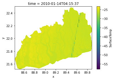
# calculate the NDVI
ds['NDVI'] = (ds.B4 - ds.B3) / (ds.B4 + ds.B3)
# find max and min values of NDVI
max_ndvi = ds.NDVI.max()
min_ndvi = ds.NDVI.min()
# print the max and min values
print(max_ndvi, min_ndvi)
# calculate the thermal band BT = (K2 / (ln (K1 / L) + 1)) − 273.15
ds['BT'] = (607.76/ (np.log(1260.56/ ds.B6) + 1)) - 273.15
# calculate the proportion of NDVI
ds['PV'] = ((ds.NDVI - -0.71949685) / (0.88091075- min_ndvi))**2
# calculate Emissivity
ds['Emissivity'] = 0.956 + 0.004 * ds.PV
# calculate the surface temperature
ds['SurfaceTemp'] = ds.BT /(1+((0.00115 *ds.BT)/1.4388)*np.log(ds.Emissivity))
# print max and min surface temperature and print them
print(ds.SurfaceTemp.max(), ds.BT.min())
<xarray.DataArray 'NDVI' ()>
array(0.88091075) <xarray.DataArray 'NDVI' ()>
array(-0.71949685)
<xarray.DataArray 'SurfaceTemp' ()>
array(-23.36428851) <xarray.DataArray 'BT' ()>
array(-57.96063232)collection = (ee.ImageCollection("MODIS/006/MOD09GA")
.filterDate("2021-06-01", "2021-06-05")
.select(["sur_refl_b01", "sur_refl_b04" ,"sur_refl_b03"])
)
# NDVI
modis = wxee.TimeSeries("MODIS/MOD09GA_006_NDVI").filterDate("2000", "2021").select('NDVI')
# LST 1000 METER
#modis = wxee.TimeSeries("MODIS/061/MOD11A1").filterDate("2000", "2021").select('LST_Day_1km')
#lst.multyply(0.02).substract(273.15)
# ts = (modis
# .maskClouds(maskShadows=False)
# .scaleAndOffset()
# .spectralIndices(index="NDVI")
# .select("NDVI")
# )
#'year', 'month' 'week', 'day', 'hour'.
monthly_ts = modis.aggregate_time("year", ee.Reducer.median())
monthly_ts<wxee.time_series.TimeSeries at 0x27f8bd3e400># Spatial resolution in CRS units (meters)
scale = 500
files = monthly_ts.wx.to_tif(
out_dir="E:\python_projects\essential_visualization",
prefix="wx_",
region=roi,
scale=30,
crs="EPSG:4326"
)
files['E:\\python_projects\\essential_visualization\\wx_MODIS_MOD09GA_006_NDVI_2000_02_24.time.20000224T000000.tif',
'E:\\python_projects\\essential_visualization\\wx_MODIS_MOD09GA_006_NDVI_2001_02_24.time.20010224T000000.tif',
'E:\\python_projects\\essential_visualization\\wx_MODIS_MOD09GA_006_NDVI_2002_02_24.time.20020224T000000.tif',
'E:\\python_projects\\essential_visualization\\wx_MODIS_MOD09GA_006_NDVI_2003_02_24.time.20030224T000000.tif',
'E:\\python_projects\\essential_visualization\\wx_MODIS_MOD09GA_006_NDVI_2004_02_24.time.20040224T000000.tif',
'E:\\python_projects\\essential_visualization\\wx_MODIS_MOD09GA_006_NDVI_2005_02_24.time.20050224T000000.tif',
'E:\\python_projects\\essential_visualization\\wx_MODIS_MOD09GA_006_NDVI_2006_02_24.time.20060224T000000.tif',
'E:\\python_projects\\essential_visualization\\wx_MODIS_MOD09GA_006_NDVI_2007_02_24.time.20070224T000000.tif',
'E:\\python_projects\\essential_visualization\\wx_MODIS_MOD09GA_006_NDVI_2008_02_24.time.20080224T000000.tif',
'E:\\python_projects\\essential_visualization\\wx_MODIS_MOD09GA_006_NDVI_2009_02_24.time.20090224T000000.tif',
'E:\\python_projects\\essential_visualization\\wx_MODIS_MOD09GA_006_NDVI_2010_02_24.time.20100224T000000.tif',
'E:\\python_projects\\essential_visualization\\wx_MODIS_MOD09GA_006_NDVI_2011_02_24.time.20110224T000000.tif',
'E:\\python_projects\\essential_visualization\\wx_MODIS_MOD09GA_006_NDVI_2012_02_24.time.20120224T000000.tif',
'E:\\python_projects\\essential_visualization\\wx_MODIS_MOD09GA_006_NDVI_2013_02_24.time.20130224T000000.tif',
'E:\\python_projects\\essential_visualization\\wx_MODIS_MOD09GA_006_NDVI_2014_02_24.time.20140224T000000.tif',
'E:\\python_projects\\essential_visualization\\wx_MODIS_MOD09GA_006_NDVI_2015_02_24.time.20150224T000000.tif',
'E:\\python_projects\\essential_visualization\\wx_MODIS_MOD09GA_006_NDVI_2016_02_28.time.20160228T000000.tif',
'E:\\python_projects\\essential_visualization\\wx_MODIS_MOD09GA_006_NDVI_2017_02_24.time.20170224T000000.tif',
'E:\\python_projects\\essential_visualization\\wx_MODIS_MOD09GA_006_NDVI_2018_02_24.time.20180224T000000.tif',
'E:\\python_projects\\essential_visualization\\wx_MODIS_MOD09GA_006_NDVI_2019_02_24.time.20190224T000000.tif',
'E:\\python_projects\\essential_visualization\\wx_MODIS_MOD09GA_006_NDVI_2020_02_24.time.20200224T000000.tif']modis = wxee.TimeSeries("MODIS/006/MOD09GA").filterDate("2020", "2021")ts = (modis
.maskClouds(maskShadows=False)
.scaleAndOffset()
.spectralIndices(index="NDVI")
.select("NDVI")
)ts<wxee.time_series.TimeSeries at 0x27f88649790>monthly_ts = ts.aggregate_time("month", ee.Reducer.median())
monthly_ts<wxee.time_series.TimeSeries at 0x27f886f88e0>monthly_ts_land = monthly_ts.map(lambda img: img.clip(roi))ds = monthly_ts_land.wx.to_xarray(region=roi, scale=50)
ds<xarray.Dataset>
Dimensions: (time: 21, y: 538, x: 318)
Coordinates:
* time (time) datetime64[ns] 2000-02-24 2001-02-24 ... 2020-02-24
* y (y) float64 22.47 22.47 22.47 22.47 ... 22.23 22.23 22.23 22.23
* x (x) float64 91.75 91.75 91.75 91.75 ... 91.89 91.89 91.89 91.89
Data variables:
NDVI (time, y, x) float32 nan nan nan nan nan ... nan nan nan nan nan
Attributes:
transform: (0.00044915764205976077, 0.0, 91.74808407062115,...
crs: +init=epsg:4326
res: (0.00044915764205976077, 0.00044915764205976077)
is_tiled: 1
nodatavals: (-32768.0,)
scales: (1.0,)
offsets: (0.0,)
AREA_OR_POINT: Area
TIFFTAG_RESOLUTIONUNIT: 1 (unitless)
TIFFTAG_XRESOLUTION: 1
TIFFTAG_YRESOLUTION: 1xarray.Dataset
- time: 21
- y: 538
- x: 318
- time(time)datetime64[ns]2000-02-24 ... 2020-02-24
array(['2000-02-24T00:00:00.000000000', '2001-02-24T00:00:00.000000000', '2002-02-24T00:00:00.000000000', '2003-02-24T00:00:00.000000000', '2004-02-24T00:00:00.000000000', '2005-02-24T00:00:00.000000000', '2006-02-24T00:00:00.000000000', '2007-02-24T00:00:00.000000000', '2008-02-24T00:00:00.000000000', '2009-02-24T00:00:00.000000000', '2010-02-24T00:00:00.000000000', '2011-02-24T00:00:00.000000000', '2012-02-24T00:00:00.000000000', '2013-02-24T00:00:00.000000000', '2014-02-24T00:00:00.000000000', '2015-02-24T00:00:00.000000000', '2016-02-28T00:00:00.000000000', '2017-02-24T00:00:00.000000000', '2018-02-24T00:00:00.000000000', '2019-02-24T00:00:00.000000000', '2020-02-24T00:00:00.000000000'], dtype='datetime64[ns]') - y(y)float6422.47 22.47 22.47 ... 22.23 22.23
array([22.46709 , 22.466641, 22.466192, ..., 22.22679 , 22.226341, 22.225892])
- x(x)float6491.75 91.75 91.75 ... 91.89 91.89
array([91.748309, 91.748758, 91.749207, ..., 91.889793, 91.890242, 91.890692])
- NDVI(time, y, x)float32nan nan nan nan ... nan nan nan nan
- transform :
- (0.00044915764205976077, 0.0, 91.74808407062115, 0.0, -0.00044915764205976077, 22.467314413471293)
- crs :
- +init=epsg:4326
- res :
- (0.00044915764205976077, 0.00044915764205976077)
- is_tiled :
- 1
- nodatavals :
- (-32768.0,)
- scales :
- (1.0,)
- offsets :
- (0.0,)
- AREA_OR_POINT :
- Area
- TIFFTAG_RESOLUTIONUNIT :
- 1 (unitless)
- TIFFTAG_XRESOLUTION :
- 1
- TIFFTAG_YRESOLUTION :
- 1
array([[[nan, nan, nan, ..., nan, nan, nan],
        [nan, nan, nan, ..., nan, nan, nan],
        [nan, nan, nan, ..., nan, nan, nan],
        ...,
        [nan, nan, nan, ..., nan, nan, nan],
        [nan, nan, nan, ..., nan, nan, nan],
        [nan, nan, nan, ..., nan, nan, nan]],

       [[nan, nan, nan, ..., nan, nan, nan],
        [nan, nan, nan, ..., nan, nan, nan],
        [nan, nan, nan, ..., nan, nan, nan],
        ...,
        [nan, nan, nan, ..., nan, nan, nan],
        [nan, nan, nan, ..., nan, nan, nan],
        [nan, nan, nan, ..., nan, nan, nan]],

       [[nan, nan, nan, ..., nan, nan, nan],
        [nan, nan, nan, ..., nan, nan, nan],
        [nan, nan, nan, ..., nan, nan, nan],
        ...,
...
        ...,
        [nan, nan, nan, ..., nan, nan, nan],
        [nan, nan, nan, ..., nan, nan, nan],
        [nan, nan, nan, ..., nan, nan, nan]],

       [[nan, nan, nan, ..., nan, nan, nan],
        [nan, nan, nan, ..., nan, nan, nan],
        [nan, nan, nan, ..., nan, nan, nan],
        ...,
        [nan, nan, nan, ..., nan, nan, nan],
        [nan, nan, nan, ..., nan, nan, nan],
        [nan, nan, nan, ..., nan, nan, nan]],

       [[nan, nan, nan, ..., nan, nan, nan],
        [nan, nan, nan, ..., nan, nan, nan],
        [nan, nan, nan, ..., nan, nan, nan],
        ...,
        [nan, nan, nan, ..., nan, nan, nan],
        [nan, nan, nan, ..., nan, nan, nan],
        [nan, nan, nan, ..., nan, nan, nan]]], dtype=float32)
- transform :
- (0.00044915764205976077, 0.0, 91.74808407062115, 0.0, -0.00044915764205976077, 22.467314413471293)
- crs :
- +init=epsg:4326
- res :
- (0.00044915764205976077, 0.00044915764205976077)
- is_tiled :
- 1
- nodatavals :
- (-32768.0,)
- scales :
- (1.0,)
- offsets :
- (0.0,)
- AREA_OR_POINT :
- Area
- TIFFTAG_RESOLUTIONUNIT :
- 1 (unitless)
- TIFFTAG_XRESOLUTION :
- 1
- TIFFTAG_YRESOLUTION :
- 1
#select time for 2000,2005,2010,2015,2020
new=ds.sel(time=['2000-01-01', '2005-01-01', '2010-01-01', '2015-01-01', '2020-01-01'])

# plot the
g=new.NDVI.plot(col='time', col_wrap=3, cmap='RdYlGn') #YlOrRd
# set the title first plot ,'2000', send '2005', '2010', '2015', '2020'
titles = ["2000", "2005", "2010", "`2015", "2020"]
for ax, title in zip(g.axes.flat, titles):
    ax.set_title(title,fontweight='bold',fontsize=12)
# axis x label 'Latitude' and y label 'Longitude'
ax.set_xlabel('Latitude',fontsize=12)
# add colorbar named 'NDVI'
cbar = g.fig.colorbar(g.collections[0], ax=g.axes, shrink=0.9)
cbar.ax.set_ylabel('NDVI',fontweight='bold',fontsize=12)
# save the figure
plt.savefig('E:\python_projects\essential_visualization\NDVI.png')

# write xarray to geotiff for loop
time=['2000-01-01', '2005-01-01', '2010-01-01', '2015-01-01', '2020-01-01']
# extract mean of NDVI for each year and convert to pandas dataframe
ndvi_mean=new.NDVI.mean(dim='time').to_pandas()

for i in time:
ds.sel(time=i).NDVI.to_geotiff('E:\python_projects\essential_visualization\NDVI_'+i+'.tif')ds.NDVI.plot(col="time", col_wrap=4, cmap="YlGn", vmin=0, vmax=1, aspect=0.8)<xarray.plot.facetgrid.FacetGrid at 0x27f8bc90b80>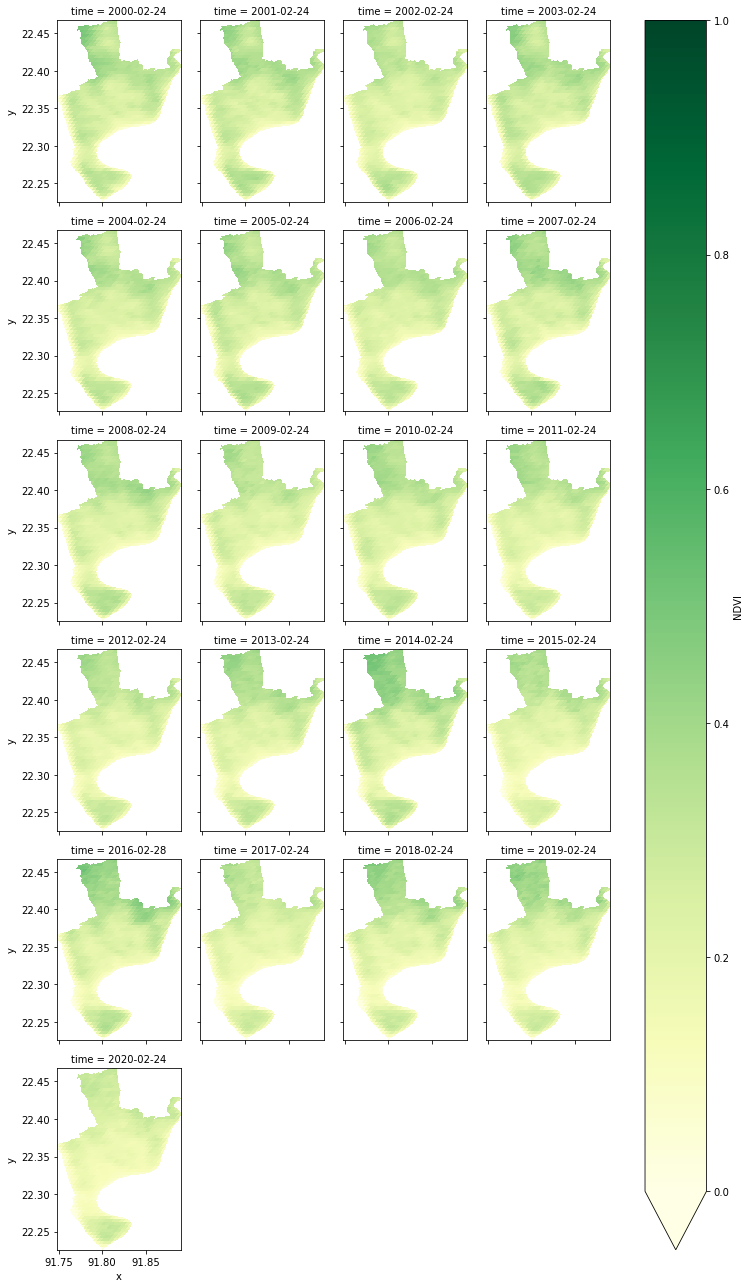
collection = wxee.TimeSeries("LANDSAT/LE07/C01/T1_SR").filterDate('2000-01-01', '2001-5-20').select(['B6'])
monthly_ts = collection.aggregate_time("month", ee.Reducer.median())
monthly_ts_land = monthly_ts.map(lambda img: img.clip(roi))
s = monthly_ts_land.wx.to_xarray(region=roi, scale=50)
ds6=ds['B6']*0.1
ds6c=ds6-273.15 # landast 7
EEException: User memory limit exceeded.#eemont.listIndices()# select time for 2000,2005,2010,2015,2020 and loop find average lst for each year
collection = wxee.TimeSeries("LANDSAT/LE07/C01/T1_SR").filterDate('2001-1-10', '2002-1-10')
monthly_ts = collection.aggregate_time("month", ee.Reducer.median())
monthly_ts_land = monthly_ts.map(lambda img: img.clip(roi))
ds = monthly_ts_land.wx.to_xarray(region=roi, scale=900)
ds6=ds['B6']*0.1
ds6c=ds6-273.15 # landast 7
time=ds6c.time.values
lst_mean=[]
for i in time:
l=ds6c.sel(time=i).mean().values
lst_mean.append(l)
df=pd.DataFrame({'lst':lst_mean,'date':time})
df.to_csv('2001lst.csv',index=False)landsat7=(ee.ImageCollection('LANDSAT/LE07/C01/T1_SR')
.filterBounds(roi)
.filterDate('2000-1-10', '2020-10-10')
.maskClouds()
.scale()
.select(['B6']))# version of eemont
print(eemont.__version__)0.3.4ts = landsat7.getTimeSeriesByRegions(reducer = [ee.Reducer.mean()],
bands = ['B6'],collection=fc,
scale = 30)L8 = (ee.ImageCollection("LANDSAT/LE07/C01/T1_8DAY_NDVI")
.filterBounds(delta)
.filterDate("2020-01-01","2020-02-01")
.preprocess()
.spectralIndices(["NDVI"])
.mean())c:\Users\Hafez\miniconda3\lib\site-packages\ee_extra\QA\clouds.py:310: UserWarning: This platform is not supported for cloud masking.
warnings.warn("This platform is not supported for cloud masking.")Exception: Sorry, satellite platform not supported for index computation!# landsat 7 land surface temperature time series
collection = wxee.TimeSeries("LANDSAT/LE07/C01/T1_SR").filterDate('2000-1-10', '2020-10-10').filterBounds(roi).select(['B3','B4'])
monthly_ts = collection.aggregate_time("year", ee.Reducer.median())
monthly_ts_land = monthly_ts.map(lambda img: img.clip(roi))ds = monthly_ts_land.wx.to_xarray(region=roi, scale=30)collection = wxee.TimeSeries("LANDSAT/LE07/C01/T1_SR").filterDate('2000-1-10', '2020-12-10').filterBounds(roi).select(['B6'])
monthly_ts = collection.aggregate_time("year", ee.Reducer.median())
monthly_ts_land = monthly_ts.map(lambda img: img.clip(roi))dslst = monthly_ts_land.wx.to_xarray(region=roi, scale=30)#LANDSAT/LT05/C01/T2_SR B6 0.1
#LANDSAT/LT05/C02/T1_L2 ST_B6 0.00341802
L8 = (ee.ImageCollection('LANDSAT/LT05/C02/T1_L2')
.filterBounds(delta)
.filterDate('1990-01-10', '2000-12-30')
.scaleAndOffset()
.select(['ST_B6']))ts = L8.getTimeSeriesByRegion(geometry = delta,
reducer = [ee.Reducer.min(),ee.Reducer.mean(),ee.Reducer.max()],
scale = 30)tsPandas = geemap.ee_to_pandas(ts)
tsPandas.shapetsPandas = geemap.ee_to_pandas(ts)
# check shape of the dataframe
tsPandas.shape
# replace -9999 with nan
tsPandas.replace(-9999, np.nan, inplace=True)
# metl dataframe
lst=pd.melt(tsPandas,id_vars=['date','reducer'],value_vars=['B6'],var_name='band',value_name='lst')
# convert date to datetime
lst['date']=pd.to_datetime(lst['date'],infer_datetime_format=True)
# multiple lst by 0.1 and subtract 273.15
lst['lst']=lst['lst']*0.1
# sort by date
lst.sort_values(by='date',inplace=True)
# select reducer=max
lst_max=lst[lst['reducer']=='max']
# date and lst and filter by date 2000
lst_max_2000=lst_max[lst_max['date']<='2000-01-01']
# write to csv lst_max_2000
lst_max_2000[['lst','date']].to_csv('E:\\my works\\delta\\data\\csv\\lst_max_landsat5_1990_2000.csv',index=False)
# select reducer=min
lst_min=lst[lst['reducer']=='min']
# date and lst and filter by date 2000
lst_min_2000=lst_min[lst_min['date']<='2000-01-01']
# write to csv lst_min_2000
lst_min_2000[['lst','date']].to_csv('E:\\my works\\delta\\data\\csv\\lst_min_landsat5_1990_2000.csv',index=False)
# select reducer=mean
lst_mean=lst[lst['reducer']=='mean']
# date and lst and filter by date 2000
lst_mean_2000=lst_mean[lst_mean['date']<='2000-01-01']
# write to csv lst_mean_2000
lst_mean_2000[['lst','date']].to_csv('E:\\my works\\delta\\data\\csv\\lst_mean_landsat5_1990_2000.csv',index=False)ds<xarray.Dataset>
Dimensions: (time: 21, y: 1039, x: 1555)
Coordinates:
* time (time) datetime64[ns] 2000-01-14T16:17:56 ... 2020-01-21T16:04:59
* y (y) float64 33.57 33.57 33.57 33.57 ... 33.29 33.29 33.29 33.29
* x (x) float64 -89.09 -89.09 -89.09 -89.09 ... -88.67 -88.67 -88.67
Data variables:
B3 (time, y, x) float64 nan nan nan nan nan ... nan nan nan nan nan
B4 (time, y, x) float64 nan nan nan nan nan ... nan nan nan nan nan
Attributes:
transform: (0.00026949458523585647, 0.0, -89.09032847102515...
crs: +init=epsg:4326
res: (0.00026949458523585647, 0.00026949458523585647)
is_tiled: 1
nodatavals: (-32768.0,)
scales: (1.0,)
offsets: (0.0,)
AREA_OR_POINT: Area
TIFFTAG_RESOLUTIONUNIT: 1 (unitless)
TIFFTAG_XRESOLUTION: 1
TIFFTAG_YRESOLUTION: 1# add variable to xarray
ds['ndvi']=(ds['B4']-ds['B3'])/(ds['B4']+ds['B3'])
ds.ndvi.max()<xarray.DataArray 'ndvi' ()> array(0.89584377)
ds.ndvi.min()<xarray.DataArray 'ndvi' ()> array(-0.64008364)
dslst=dslst['B6']*0.1
ds6c=dslst-273.15 # landast 7
time=ds6c.time.values
# print max and min of lst
print(ds6c.max())
print(ds6c.min())<xarray.DataArray 'B6' ()>
array(35.95)
<xarray.DataArray 'B6' ()>
array(-2.6)time=ds.time.valuesyear=ds6c.time.dt.year.values.tolist()
year[1]2001collection = ee.ImageCollection('LANDSAT/LC08/C01/T1_TOA') \
.filterBounds(delta) \
.filterDate('2020-01-01', '2021-01-01')
collection.size().getInfo()
image = collection.median().clip(delta)# facet plot , layout 7*3
g=ds6c.plot(col="time", col_wrap=7, vmin=-2.9, vmax=36, cmap='jet', figsize=(25,8))
for i, ax in enumerate(g.axes.flat):
ax.set_title(ds6c.time.dt.year.values.tolist()[i])
ax.set_xticks([])
ax.set_xlabel('')
ax.set_ylabel('')
ax.set_yticks([])
# reduce grid space between subplots
# label colorbar
g.cbar.ax.tick_params(labelsize=25)
g.cbar.set_label(label='Land surface temperature (°C)', size=15, weight='bold')
# save figure
plt.savefig('E:/my works/starkville lulc/figure/landsat7_lst_map.png', dpi=400, bbox_inches='tight')
plt.show() 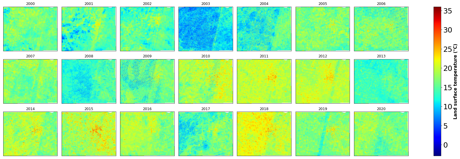
# facet plot , layout 7*3
g=ds6c.plot(col="time", col_wrap=7, vmin=12, vmax=32, cmap='jet', subplot_kws={'projection': ccrs.Robinson()})
for i, ax in enumerate(g.axes.flat):
    ax.set_title(ds6c.time.dt.year.values.tolist()[i])
    ax.coastlines()
    ax.add_feature(cfeature.BORDERS.with_scale('50m'), linewidth=0.5, edgecolor='black')
    # reduce space between subplots
    ax.set_xticks([])
    ax.set_xlabel('')
    ax.set_ylabel('')
    ax.set_yticks([])
    # reduce grid space between subplots
    # label colorbar
    g.cbar.ax.tick_params(labelsize=25)
    g.cbar.set_label(label='Land surface temperature (°C)', size=15, weight='bold')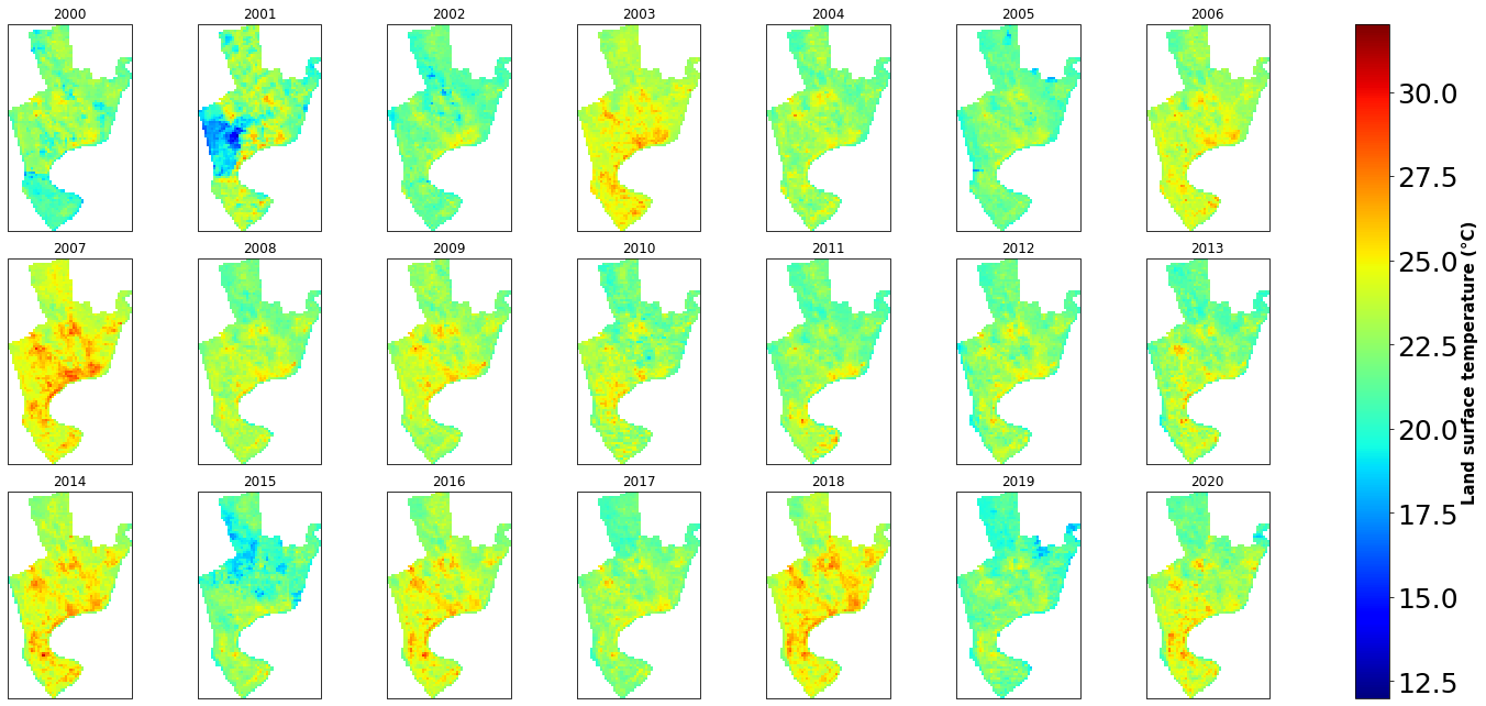
ds6c.sel(time='2000-02-05').plot(ax=ax, vmin=12, vmax=32, cmap='jet')<cartopy.mpl.geocollection.GeoQuadMesh at 0x1b5c36d6790># make subplot 7*3
fig, axes = plt.subplots(nrows=3, ncols=7,figsize=(20,10), subplot_kw=dict(projection=ccrs.Robinson()))
# plot using for loop
for i, ax in enumerate(axes.flat):
im=ds6c.sel(time=time[i]).plot(ax=ax, vmin=12, vmax=32, cmap='jet',add_colorbar=False)
ax.set_title(ds6c.time.dt.year.values.tolist()[i], fontdict={'fontsize':12},fontweight='bold')
# remove ylabel, xlabel
ax.set_ylabel('')
ax.set_xlabel('')
# remove grid
ax.grid(False)
# remove ticks
ax.set_xticks([])
ax.set_yticks([])
fig.subplots_adjust(right=0.8, top=0.9, bottom=0.1, hspace=0.1, wspace=0)
cbar_ax = fig.add_axes([0.82, 0.12, 0.05, 0.78])
# add colorbar named 'Land surface temperature'
cbar = fig.colorbar(im, cax=cbar_ax, orientation='vertical')
cbar.set_label('Land surface temperature (°C)', size=15, weight='bold')
# save figure
fig.savefig('E:/my works/land use coastal zone/ctg/figure map/landsat7_lst_map.png', dpi=400, bbox_inches='tight')
plt.show() 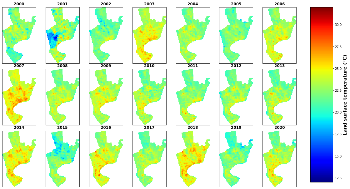
# change directory to  E:\my works\delta\data\NDVI
os.chdir('E:\\my works\\delta\\data\\NDBI')
# find all files in the directory
files=glob.glob('*.tif')
print(files)
['NDBI1990.tif', 'NDBI1995.tif', 'NDBI2000.tif', 'NDBI2005.tif', 'NDBI2010.tif', 'NDBI2015.tif', 'NDBI2020.tif']# change directory to E:\my works\delta\data\NDVI
os.chdir("E:\\1 Master's\\MSU\course classes\\2Summer 2022\\remote sensing\\project\\data\\LST")
# find all files in the directory
files=glob.glob('*.tif')
print(files)['lst1985.tif', 'lst1997.tif', 'lst2009.tif', 'lst2021.tif']ds1=rioxarray.open_rasterio(files[0])
ds1.squeeze().plot.imshow()<matplotlib.image.AxesImage at 0x17fb6375d30>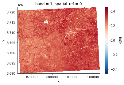
# open the first file in the directory and plot
plt.subplot(2,3,1)
ds1=rioxarray.open_rasterio(files[0])
# no xlabel, ylabel,
ds1.plot(cmap='RdYlGn')
plt.xlabel('')
plt.ylabel('')
# No grid
plt.grid(False)
# no  ticks
plt.xticks([])
plt.yticks([])
plt.title('NDVI of '+files[0][4:8],fontdict={'fontsize':12},fontweight='bold')
plt.subplot(2,3,2)
ds2=rioxarray.open_rasterio(files[1])
ds2.plot(cmap='RdYlGn')
plt.xlabel('')
plt.ylabel('')
plt.grid(False)
plt.xticks([])
plt.yticks([])
plt.title('NDVI of '+files[1][4:8],fontdict={'fontsize':12},fontweight='bold')
plt.subplot(2,3,3)
ds3=rioxarray.open_rasterio(files[2])
ds3.plot(cmap='RdYlGn')
plt.xlabel('')
plt.ylabel('')
plt.grid(False)
plt.xticks([])
plt.yticks([])
plt.title('NDVI of '+files[2][4:8],fontdict={'fontsize':12},fontweight='bold')
plt.subplot(2,3,4)
ds4=rioxarray.open_rasterio(files[3])
Text(0.5, 1.0, 'NDVI of 1990')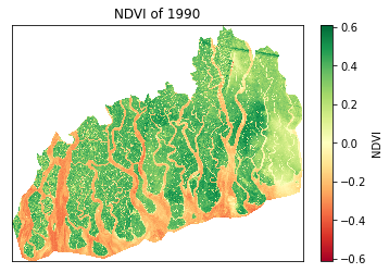
# change directory to  E:\my works\delta\data\NDVI
os.chdir("E:/1 Master's/MSU/course classes/2Summer 2022/remote sensing/project/data/ndvi")
# find all files in the directory
files=glob.glob('*.tif')
print(files)
# find all max and min value of NDVI for each file
for i in range (0,4):
    ds=rioxarray.open_rasterio(files[i])
    # find max and min value of NDVI
    print(f"NDVI of  {files[i][4:8]}, min: {ds.min().values:,.2f}, and mean: {ds.mean().values:,.2f}, and max: {ds.max().values:,.2f}")
os.chdir("E:/1 Master's/MSU/course classes/2Summer 2022/remote sensing/project/data/LST")
# find all files in the directory
files=glob.glob('*.tif')
print(files)
# find all max and min value of NDVI for each file
for i in range(0,4):
    ds=rioxarray.open_rasterio(files[i])
    # filter the data remove the values less than 0
    ds=ds.where(ds>-3)
    # find max and min value of NDVI
    print(f"LST of {files[i][3:7]}, min: {ds.min().values:,.2f}, and mean: {ds.mean().values:,.2f}, and max: {ds.max().values:,.2f}")
['ndvi1985.tif', 'ndvi1997.tif', 'ndvi2009.tif', 'ndvi2021.tif']
NDVI of 1985, min: -0.12, and mean: 0.28, and max: 0.46
NDVI of 1997, min: -0.10, and mean: 0.28, and max: 0.42
NDVI of 2009, min: -0.12, and mean: 0.29, and max: 0.46
NDVI of 2021, min: -0.77, and mean: 0.70, and max: 0.96
['LST1985_C.tif', 'lst1997.tif', 'lst2009.tif', 'lst2021.tif']
LST of 1985, min: -2.27, and mean: 19.09, and max: 30.86
LST of 1997, min: 8.17, and mean: 16.21, and max: 25.58
LST of 2009, min: 6.06, and mean: 16.31, and max: 30.67
LST of 2021, min: 12.53, and mean: 18.86, and max: 32.76files[1][4:8]'1997'# make subplot 2 row and 2 column
fig, axs = plt.subplots(2, 2, figsize=(25,10))
for i, ax in enumerate(axs.flat):
ds=rioxarray.open_rasterio(files[i])
# no xlabel, ylabel,
im=ds.squeeze().plot.imshow(ax=ax, vmin=-0.77, vmax=0.9, cmap='Greens',add_colorbar=False)
ax.set_title(files[i][4:8],fontdict={'fontsize':20},fontweight='bold')
# remove xlabel, ylabel
ax.set_xlabel('')
ax.set_ylabel('')
ax.set_xticks([])
ax.set_yticks([])
# remove grid
ax.grid(False)
fig.subplots_adjust(right=0.8, top=0.9, bottom=0.1, hspace=0.1, wspace=0)
cbar_ax = fig.add_axes([0.82, 0.12, 0.05, 0.78])
# add colorbar named 'Land surface temperature'
cbar = fig.colorbar(im, cax=cbar_ax, orientation='vertical')
cbar.set_label('Normalized Difference Vegetation Index', size=15, weight='bold')
# save as jpeg
fig.savefig("E:\\1 Master's\\MSU\\course classes\\2Summer 2022\\remote sensing\\project\\figure\\ndvi_map.jpg", dpi=400, bbox_inches='tight')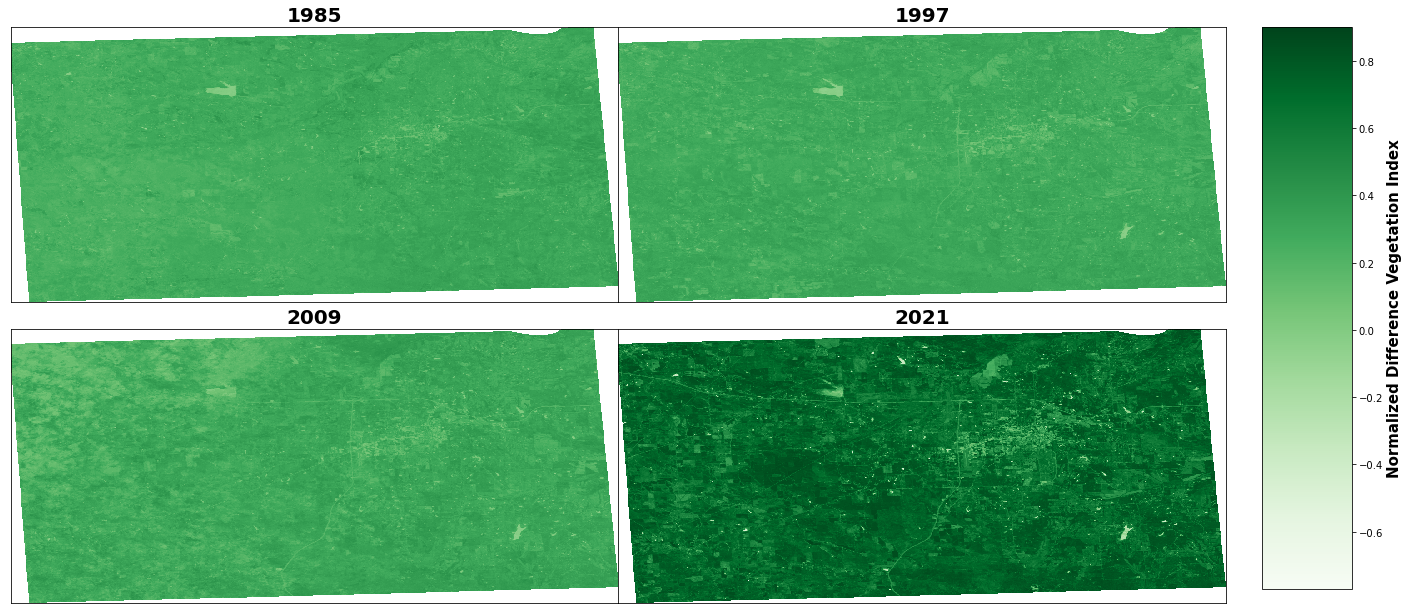
# change directory to  E:\my works\delta\data\NDVI
os.chdir("E:/1 Master's/MSU/course classes/2Summer 2022/remote sensing/project/data/LST")
# find all files in the directory
files=glob.glob('*.tif')
# make subplot 2 row and 2 column
fig, axs = plt.subplots(2, 2, figsize=(25,10))
for i, ax in enumerate(axs.flat):
    ds=rioxarray.open_rasterio(files[i])
    # no xlabel, ylabel,
    im=ds.squeeze().plot.imshow(ax=ax, vmin=-2, vmax=33, cmap='jet',add_colorbar=False)
    ax.set_title(files[i][3:7],fontdict={'fontsize':20},fontweight='bold')
    # remove xlabel, ylabel
    ax.set_xlabel('')
    ax.set_ylabel('')
    ax.set_xticks([])
    ax.set_yticks([])
    # remove grid
    ax.grid(False)
fig.subplots_adjust(right=0.8, top=0.9, bottom=0.1, hspace=0.1, wspace=0)
cbar_ax = fig.add_axes([0.82, 0.12, 0.05, 0.78])
# add colorbar named 'Land surface temperature'
cbar = fig.colorbar(im, cax=cbar_ax, orientation='vertical')
cbar.set_label('Land surface temperature(C)', size=15, weight='bold')
# save as jpeg
fig.savefig("E:\\1 Master's\\MSU\\course classes\\2Summer 2022\\remote sensing\\project\\figure\\lst_map.jpg", dpi=400, bbox_inches='tight')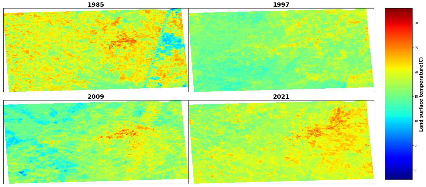
# make subplot row=2, col=3
fig, axes = plt.subplots(nrows=2, ncols=4,figsize=(20,10))
# plot using for loop
for i, ax in enumerate(axes.flat):
    # break the loop when i=7
    if i==7:
        break
    # open the file
    # open the first file in the directory and plot
    ds=rioxarray.open_rasterio(files[i])
    # no xlabel, ylabel,
    im=ds.squeeze().plot.imshow(ax=ax, vmin=-0.9, vmax=0, cmap='jet',add_colorbar=False)
    ax.set_title(files[i][4:8],fontdict={'fontsize':12},fontweight='bold')
    # remove xlabel, ylabel
    ax.set_xlabel('')
    ax.set_ylabel('')
    ax.set_xticks([])
    ax.set_yticks([])
    # remove grid
    ax.grid(False)
fig.subplots_adjust(right=0.8, top=0.9, bottom=0.1, hspace=0.1, wspace=0)
cbar_ax = fig.add_axes([0.82, 0.12, 0.05, 0.78])
# add colorbar named 'Land surface temperature'
cbar = fig.colorbar(im, cax=cbar_ax, orientation='vertical')
cbar.set_label('Normalized Difference Built-Up Index', size=15, weight='bold')
# delete last subplot
fig.delaxes(axes[1,3])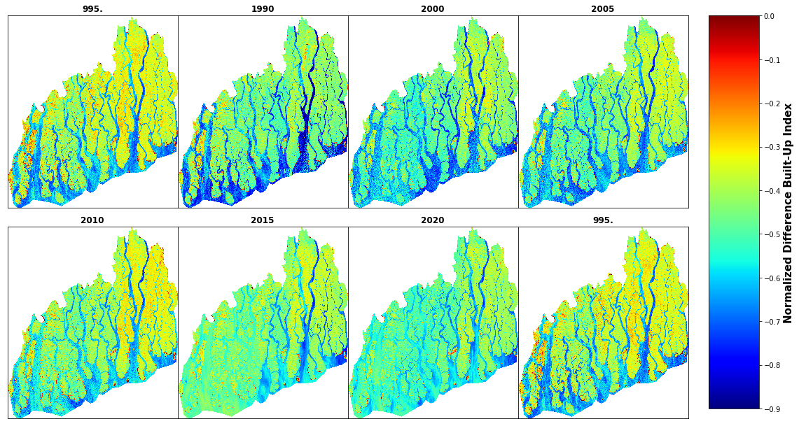
# make subplot row=2, col=3
fig, axes = plt.subplots(nrows=2, ncols=4,figsize=(20,10))
# plot using for loop
for i, ax in enumerate(axes.flat):
    # open the first file in the directory and plot
    ds=rioxarray.open_rasterio(files[i-1])
    # no xlabel, ylabel,
    im=ds.squeeze().plot.imshow(ax=ax, vmin=-0.8, vmax=0.9, cmap='RdYlGn',add_colorbar=False)
    ax.set_title(files[i-1][4:8],fontdict={'fontsize':12},fontweight='bold')
    # remove xlabel, ylabel
    ax.set_xlabel('')
    ax.set_ylabel('')
    ax.set_xticks([])
    ax.set_yticks([])
    # remove grid
    ax.grid(False)
    i+=1
fig.subplots_adjust(right=0.8, top=0.9, bottom=0.1, hspace=0.1, wspace=0)
cbar_ax = fig.add_axes([0.82, 0.12, 0.05, 0.78])
# add colorbar named 'Land surface temperature'
cbar = fig.colorbar(im, cax=cbar_ax, orientation='vertical')
cbar.set_label('Normalized difference vegetation index', size=15, weight='bold')
# save figure
#fig.savefig('landsat_ndvi_map.png', dpi=400, bbox_inches='tight')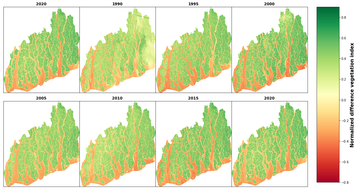
# make subplot 7*3
fig, axes = plt.subplots(nrows=3, ncols=7,figsize=(20,10), subplot_kw=dict(projection=ccrs.Robinson()))
# plot using for loop
for i, ax in enumerate(axes.flat):
    im=ds.sel(time=time[i]).ndvi.plot(ax=ax, vmin=-0.6, vmax=0.8, cmap='RdYlGn',add_colorbar=False)
    ax.set_title(ds.time.dt.year.values.tolist()[i], fontdict={'fontsize':12},fontweight='bold')
    # remove ylabel, xlabel
    ax.set_ylabel('')
    ax.set_xlabel('')
    # remove grid
    ax.grid(False)
    # remove ticks
    ax.set_xticks([])
    ax.set_yticks([])

fig.subplots_adjust(right=0.8, top=0.9, bottom=0.1, hspace=0.1, wspace=0)
cbar_ax = fig.add_axes([0.82, 0.12, 0.05, 0.78])
# add colorbar named 'Land surface temperature'
cbar = fig.colorbar(im, cax=cbar_ax, orientation='vertical')
cbar.set_label('Normalized difference vegetation index', size=15, weight='bold')
# save figure
fig.savefig('E:/my works/land use coastal zone/ctg/figure map/landsat7_ndvi_map.png', dpi=400, bbox_inches='tight')
plt.show() 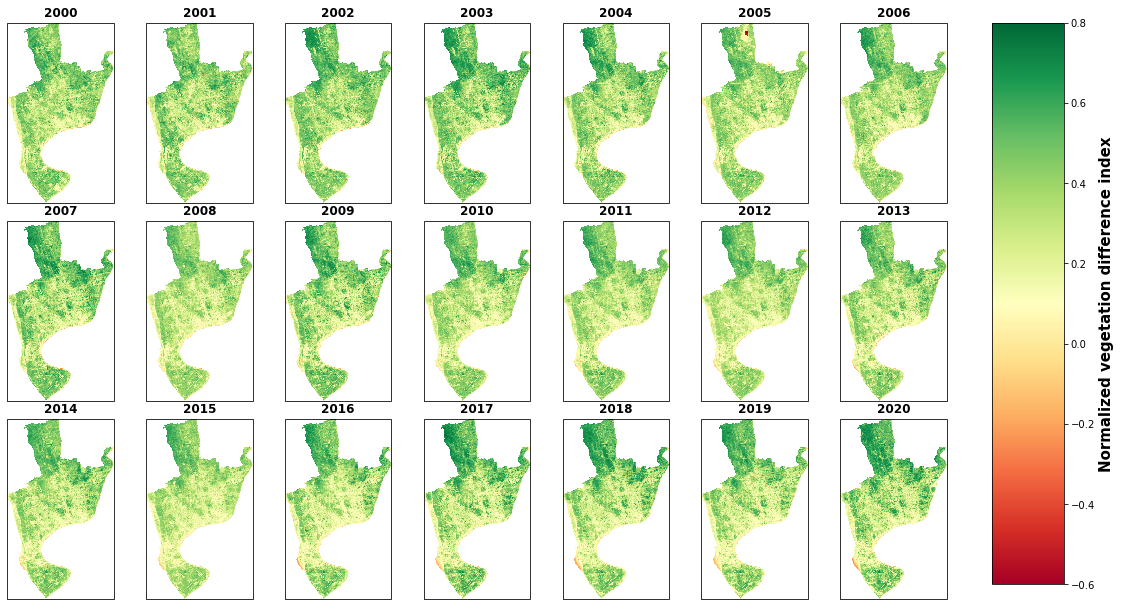
g=ds.ndvi.plot(col="time", col_wrap=7, vmin=-0.64, vmax=0.9, cmap='RdYlGn', figsize=(25,8))
for i, ax in enumerate(g.axes.flat):
    ax.set_title(ds.time.dt.year.values.tolist()[i])
    # reduce space between subplots
    ax.set_xticks([])
    ax.set_xlabel('')
    ax.set_ylabel('')
    ax.set_yticks([])
    # reduce grid space between subplots
    # label colorbar
    g.cbar.ax.tick_params(labelsize=25)
    g.cbar.set_label('Normalized vegetation difference index', size=15, weight='bold')
# save figure
# save figure
plt.savefig('E:/my works/starkville lulc/figure/landsat7_ndvi_map.png', dpi=400, bbox_inches='tight')
plt.show() 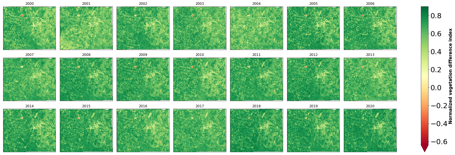
# make subplot 7*3
fig, axes = plt.subplots(nrows=3, ncols=7,figsize=(20,10), subplot_kw=dict(projection=ccrs.Robinson()))
# plot using for loop
for i, ax in enumerate(axes.flat):
    im=ds.sel(time=time[i]).ndvi.plot(ax=ax, vmin=-0.6, vmax=0.8, cmap='RdYlGn',add_colorbar=False)
    ax.set_title(ds.time.dt.year.values.tolist()[i], fontdict={'fontsize':12},fontweight='bold')
    # remove ylabel, xlabel
    ax.set_ylabel('')
    ax.set_xlabel('')
    # remove grid
    ax.grid(False)
    # remove ticks
    ax.set_xticks([])
    ax.set_yticks([])

fig.subplots_adjust(right=0.8, top=0.9, bottom=0.1, hspace=0.1, wspace=0)
cbar_ax = fig.add_axes([0.82, 0.12, 0.05, 0.78])
# add colorbar named 'Land surface temperature'
cbar = fig.colorbar(im, cax=cbar_ax, orientation='vertical')
cbar.set_label('Normalized vegetation difference index', size=15, weight='bold')
# save figure
fig.savefig('E:/my works/starkville lulc/figure/landsat7_ndvi_map.png', dpi=400, bbox_inches='tight')
plt.show() 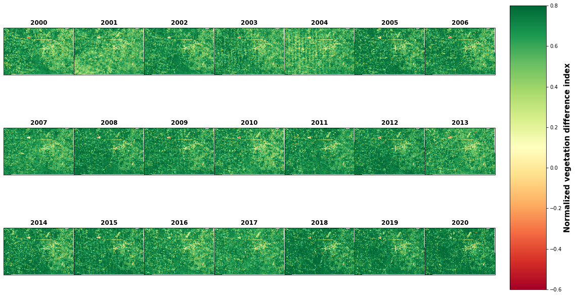
ds.ndvi.max()<xarray.DataArray 'ndvi' ()> array(0.81266968)
import hvplot.xarray
import holoviews as hvhv.extension("bokeh")
ds.NDVI.hvplot(
groupby="time", clim=(0, 1), cmap="YlGn",
frame_height=600, aspect=0.8,
widget_location="bottom", widget_type="scrubber",
)

Unable to display output for mime type(s): Unable to display output for mime type(s): os.chdir('E:\my works\land use coastal zone\ctg\Data\LST')files=['LST2000.tif', 'LST2005.tif','LST2010.tif','LST2015.tif','LST2020.tif']
chunk=5
rastterlist=[xr.open_rasterio(x,chunks={'x':None,'y':None}) for x in files]C:\Users\Hafez\AppData\Local\Temp\ipykernel_11588\951139861.py:3: DeprecationWarning: open_rasterio is Deprecated in favor of rioxarray. For information about transitioning, see: https://corteva.github.io/rioxarray/stable/getting_started/getting_started.html
rastterlist=[xr.open_rasterio(x,chunks={'x':None,'y':None}) for x in files]rastters=xr.concat(rastterlist,dim='band')
rastters<xarray.DataArray (band: 5, y: 889, x: 491)>
dask.array<concatenate, shape=(5, 889, 491), dtype=float32, chunksize=(1, 889, 491), chunktype=numpy.ndarray>
Coordinates:
* band (band) int64 1 1 1 1 1
* y (y) float64 2.485e+06 2.485e+06 2.485e+06 ... 2.458e+06 2.458e+06
* x (x) float64 3.711e+05 3.712e+05 3.712e+05 ... 3.858e+05 3.858e+05
Attributes:
transform: (30.0, 0.0, 371115.0, 0.0, -30.0, 2485005.0)
crs: +init=epsg:32646
res: (30.0, 30.0)
is_tiled: 0
nodatavals: (-3.3999999521443642e+38,)
scales: (1.0,)
offsets: (0.0,)
AREA_OR_POINT: Areagsw = ee.Image('JRC/GSW1_1/GlobalSurfaceWater')
print(gsw.bandNames().getInfo())['occurrence', 'change_abs', 'change_norm', 'seasonality', 'recurrence', 'transition', 'max_extent']occurrence = gsw.select('occurrence')
vis_occurrence = {'min': 0, 'max': 100, 'palette': ['red', 'blue']}
water_mask = occurrence.gt(90).selfMask()
vis_water_mask = {'palette': ['white', 'blue']}
Map = geemap.Map()
Map.add_basemap('HYBRID')
MapMap.setCenter(-90.98, 32.49, 11)
Map.addLayer(water_mask, vis_water_mask, 'Water Mask (>90%)')js='''
var length = myjrc.size();
var list = myjrc.toList(length);
var image_name=ee.Image(list.get(1))
'''
geemap.js_snippet_to_py(js)import ee
import geemap
jrc = ee.ImageCollection("JRC/GSW1_0/MonthlyHistory")
# Define study period
startDate = ee.Date.fromYMD(1985, 1, 1)
endDate = ee.Date.fromYMD(1986, 12, 31)
# Compute a median image and display.
# filter jrc data for country and period
myjrc = jrc.filterBounds(lmav).filterDate(startDate, endDate)
# get the size of the collection and cast colelciton to a listdates=myjrc.aggregate_array('system:index').getInfo()
# export each to google drive for loop dates in description
count=int(myjrc.size().getInfo())
print(count)
for i in range(0,count):
image=ee.Image(myjrc.toList(count).get(i))
names=dates[i]
# export to google drive
task = ee.batch.Export.image.toDrive(image, description=names, folder='google_ras',maxPixels=1e13,fileFormat='GeoTIFF',crs='EPSG:4326',scale=30,region=lmav)
task.start()'1985_04'collection = ee.ImageCollection('LANDSAT/LT05/C01/T1_TOA') \
.filterBounds(delta) \
.filterDate('1-01-01', '2000-04-28')
collection.size().getInfo()
image = collection.median().clip(delta).unmask()geemap.ee_export_image_to_drive(image,description='landsat2000',region=delta,max_pixels=1e13,folder='google_ras',file_format='GeoTIFF',scale=30)Exporting landsat2000 ...geemap.ee_export_image_collection_to_drive(image,max_pixels=1e13,folder='google_ras',file_format='GeoTIFF',scale=30)The ee_object must be an ee.ImageCollection.Map = geemap.Map()
ndwiViz = {'min': 1, 'max': 37, 'palette': ['00FFFF', '0000FF']}
Map.setCenter(89.43512348012679,22.095772163889887, 10) # San Francisco Bay
Map.add_basemap('HYBRID')
MapL5 = (ee.ImageCollection("LANDSAT/LE07/C01/T2_SR")
.filterBounds(delta)
.filterDate("2000-01-01","2001-01-01")
.preprocess()
.select(['B6'])
.median())#LANDSAT/LE07/C01/T2_SR
collection = ee.ImageCollection('LANDSAT/LE07/C01/T2_SR') \
.filterBounds(delta) \
.filterDate('2020-01-01', '2020-03-01') \
.select(['B6'])\
.median()image = collection.clip(delta)Map.addLayer(image,{"min":0,"max":3000,'palette': ['006633', 'E5FFCC', '662A00', 'D8D8D8', 'F5F5F5']},'lst')import ee
ee.Initialize()
# ====================================================================================================#
# INPUT
# ====================================================================================================#
# --------------------------------------------------
# User Requirements
# --------------------------------------------------
select_parameters = ['LST']
select_metrics = ['mean']
percentiles = []
# Time
year_start = 1990
year_end = 1990
month_start = 1
month_end = 4
# Space
select_roi = delta
max_cloud_cover = 30
epsg = 'EPSG:4326'
pixel_resolution = 30
roi_filename = 'MRD'
# --------------------------------------------------
# Algorithm Specifications
# --------------------------------------------------
ndvi_v = 0.6
ndvi_s = 0.2
epsilon_v = 0.985
epsilon_s = 0.97
epsilon_w = 0.99
t_threshold = 8
# Jiménez‐Muñoz et al. (2009) (TM & ETM+) TIGR1761 and Jiménez‐Muñoz et al. (2014) OLI-TIRS GAPRI4838
cs_l8 = [0.04019, 0.02916, 1.01523,
-0.38333, -1.50294, 0.20324,
0.00918, 1.36072, -0.27514]
cs_l7 = [0.06518, 0.00683, 1.02717,
-0.53003, -1.25866, 0.10490,
-0.01965, 1.36947, -0.24310]
cs_l5 = [0.07518, -0.00492, 1.03189,
-0.59600, -1.22554, 0.08104,
-0.02767, 1.43740, -0.25844]
# ====================================================================================================#
# FUNCTIONS
# ====================================================================================================#
lookup_metrics = {
'mean': ee.Reducer.mean(),
'min': ee.Reducer.min(),
'max': ee.Reducer.max(),
'std': ee.Reducer.stdDev(),
'median': ee.Reducer.median(),
'ts': ee.Reducer.sensSlope()
}
# --------------------------------------------------
# RENAME BANDS
# --------------------------------------------------
def fun_bands_l57(img):
bands = ['B1', 'B2', 'B3', 'B4', 'B5', 'B7']
thermal_band = ['B6']
new_bands = ['B', 'G', 'R', 'NIR', 'SWIR1', 'SWIR2']
new_thermal_bands = ['TIR']
vnirswir = img.select(bands).multiply(0.0001).rename(new_bands)
tir = img.select(thermal_band).multiply(0.1).rename(new_thermal_bands)
return vnirswir.addBands(tir).copyProperties(img, ['system:time_start'])
def fun_bands_l8(img):
bands = ['B2', 'B3', 'B4', 'B5', 'B6', 'B7']
thermal_band = ['B10']
new_bands = ['B', 'G', 'R', 'NIR', 'SWIR1', 'SWIR2']
new_thermal_bands = ['TIR']
vnirswir = img.select(bands).multiply(0.0001).rename(new_bands)
tir = img.select(thermal_band).multiply(0.1).rename(new_thermal_bands)
return vnirswir.addBands(tir).copyProperties(img, ['system:time_start'])
# --------------------------------------------------
# MASKING
# --------------------------------------------------
# Function to cloud mask Landsat TM, ETM+, OLI_TIRS Surface Reflectance Products
def fun_mask_ls_sr(img):
cloudShadowBitMask = ee.Number(2).pow(3).int()
cloudsBitMask = ee.Number(2).pow(5).int()
snowBitMask = ee.Number(2).pow(4).int()
qa = img.select('pixel_qa')
mask = qa.bitwiseAnd(cloudShadowBitMask).eq(0).And(
qa.bitwiseAnd(cloudsBitMask).eq(0)).And(
qa.bitwiseAnd(snowBitMask).eq(0))
return img.updateMask(mask)
# Function to mask LST below certain temperature threshold
def fun_mask_T(img):
mask = img.select('LST').gt(t_threshold)
return img.updateMask(mask)
# --------------------------------------------------
# MATCHING AND CALIBRATION
# --------------------------------------------------
# Radiometric Calibration
def fun_radcal(img):
radiance = ee.Algorithms.Landsat.calibratedRadiance(img).rename('RADIANCE')
return img.addBands(radiance)
# L to ee.Image
def fun_l_addband(img):
l = ee.Image(img.get('L')).select('RADIANCE').rename('L')
return img.addBands(l)
# Create maxDifference-filter to match TOA and SR products
maxDiffFilter = ee.Filter.maxDifference(
difference=2 * 24 * 60 * 60 * 1000,
leftField= 'system:time_start',
rightField= 'system:time_start'
)
# Define join: Water vapor
join_wv = ee.Join.saveBest(
matchKey = 'WV',
measureKey = 'timeDiff'
)
# Define join: Radiance
join_l = ee.Join.saveBest(
matchKey = 'L',
measureKey = 'timeDiff'
)
# --------------------------------------------------
# PARAMETER CALCULATION
# --------------------------------------------------
# NDVI
def fun_ndvi(img):
ndvi = img.normalizedDifference(['NIR', 'R']).rename('NDVI')
return img.addBands(ndvi)
def fun_ndwi(img):
ndwi = img.normalizedDifference(['NIR', 'SWIR1']).rename('NDWI')
return img.addBands(ndwi)
# Tasseled Cap Transformation (brightness, greenness, wetness) based on Christ (1985)
def fun_tcg(img):
tcg = img.expression(
'B*(-0.1603) + G*(-0.2819) + R*(-0.4934) + NIR*0.7940 + SWIR1*(-0.0002) + SWIR2*(-0.1446)',
{
'B': img.select(['B']),
'G': img.select(['G']),
'R': img.select(['R']),
'NIR': img.select(['NIR']),
'SWIR1': img.select(['SWIR1']),
'SWIR2': img.select(['SWIR2'])
}).rename('TCG')
return img.addBands(tcg)
def fun_tcb(img):
tcb = img.expression(
'B*0.2043 + G*0.4158 + R*0.5524 + NIR*0.5741 + SWIR1*0.3124 + SWIR2*0.2303',
{
'B': img.select(['B']),
'G': img.select(['G']),
'R': img.select(['R']),
'NIR': img.select(['NIR']),
'SWIR1': img.select(['SWIR1']),
'SWIR2': img.select(['SWIR2'])
}).rename('TCB')
return img.addBands(tcb)
def fun_tcw(img):
tcw = img.expression(
'B*0.0315 + G*0.2021 + R*0.3102 + NIR*0.1594 + SWIR1*(-0.6806) + SWIR2*(-0.6109)',
{
'B': img.select(['B']),
'G': img.select(['G']),
'R': img.select(['R']),
'NIR': img.select(['NIR']),
'SWIR1': img.select(['SWIR1']),
'SWIR2': img.select(['SWIR2'])
}).rename('TCW')
return img.addBands(tcw)
# Fraction Vegetation Cover (FVC)
def fun_fvc(img):
fvc = img.expression(
'((NDVI-NDVI_s)/(NDVI_v-NDVI_s))**2',
{
'NDVI': img.select('NDVI'),
'NDVI_s': ndvi_s,
'NDVI_v': ndvi_v
}
).rename('FVC')
return img.addBands(fvc)
# Scale Emissivity (Epsilon) between NDVI_s and NDVI_v
def fun_epsilon_scale(img):
epsilon_scale = img.expression(
'epsilon_s+(epsilon_v-epsilon_s)*FVC',
{
'FVC': img.select('FVC'),
'epsilon_s': epsilon_s,
'epsilon_v': epsilon_v
}
).rename('EPSILON_SCALE')
return img.addBands(epsilon_scale)
# Emissivity (Epsilon)
def fun_epsilon(img):
pseudo = img.select(['NDVI']).set('system:time_start', img.get('system:time_start'))
epsilon = pseudo.where(img.expression('NDVI > NDVI_v',
{'NDVI': img.select('NDVI'),
'NDVI_v': ndvi_v}), epsilon_v)
epsilon = epsilon.where(img.expression('NDVI < NDVI_s && NDVI >= 0',
{'NDVI': img.select('NDVI'),
'NDVI_s': ndvi_s}), epsilon_s)
epsilon = epsilon.where(img.expression('NDVI < 0',
{'NDVI': img.select('NDVI')}), epsilon_w)
epsilon = epsilon.where(img.expression('NDVI <= NDVI_v && NDVI >= NDVI_s',
{'NDVI': img.select('NDVI'),
'NDVI_v': ndvi_v,
'NDVI_s': ndvi_s}), img.select('EPSILON_SCALE')).rename('EPSILON')
return img.addBands(epsilon)
# Function to scale WV content product
def fun_wv_scale(img):
wv_scaled = ee.Image(img.get('WV')).multiply(0.1).rename('WV_SCALED')
wv_scaled = wv_scaled.resample('bilinear')
return img.addBands(wv_scaled)
# --------------------------------------------------
# LAND SURFACE TEMPERATURE CALCULATION
# --------------------------------------------------
# Atmospheric Functions
def fun_af1(cs):
def wrap(img):
af1 = img.expression(
'('+str(cs[0])+'*(WV**2))+('+str(cs[1])+'*WV)+('+str(cs[2])+')',
{
'WV': img.select('WV_SCALED')
}
).rename('AF1')
return img.addBands(af1)
return wrap
def fun_af2(cs):
def wrap(img):
af2 = img.expression(
'('+str(cs[3])+'*(WV**2))+('+str(cs[4])+'*WV)+('+str(cs[5])+')',
{
'WV': img.select('WV_SCALED')
}
).rename('AF2')
return img.addBands(af2)
return wrap
def fun_af3(cs):
def wrap(img):
af3 = img.expression(
'('+str(cs[6])+'*(WV**2))+('+str(cs[7])+'*WV)+('+str(cs[8])+')',
{
'WV': img.select('WV_SCALED')
}
).rename('AF3')
return img.addBands(af3)
return wrap
# Gamma Functions
def fun_gamma_l8(img):
gamma = img.expression('(BT**2)/(1324*L)',
{'BT': img.select('TIR'),
'L': img.select('L')
}).rename('GAMMA')
return img.addBands(gamma)
def fun_gamma_l7(img):
gamma = img.expression('(BT**2)/(1277*L)',
{'BT': img.select('TIR'),
'L': img.select('L')
}).rename('GAMMA')
return img.addBands(gamma)
def fun_gamma_l5(img):
gamma = img.expression('(BT**2)/(1256*L)',
{'BT': img.select('TIR'),
'L': img.select('L')
}).rename('GAMMA')
return img.addBands(gamma)
# Delta Functions
def fun_delta_l8(img):
delta = img.expression('BT-((BT**2)/1324)',
{'BT': img.select('TIR')
}).rename('DELTA')
return img.addBands(delta)
def fun_delta_l7(img):
delta = img.expression('BT-((BT**2)/1277)',
{'BT': img.select('TIR')
}).rename('DELTA')
return img.addBands(delta)
def fun_delta_l5(img):
delta = img.expression('BT-((BT**2)/1256)',
{'BT': img.select('TIR')
}).rename('DELTA')
return img.addBands(delta)
# Land Surface Temperature
def fun_lst(img):
lst = img.expression(
'(GAMMA*(((1/EPSILON)*(AF1*L+AF2))+AF3)+DELTA)-273.15',
{
'GAMMA': img.select('GAMMA'),
'DELTA': img.select('DELTA'),
'EPSILON': img.select('EPSILON'),
'AF1': img.select('AF1'),
'AF2': img.select('AF2'),
'AF3': img.select('AF3'),
'L': img.select('L')
}
).rename('LST')
return img.addBands(lst)
def fun_mask_lst(img):
mask = img.select('LST').gt(t_threshold)
return img.updateMask(mask)
# --------------------------------------------------
# MOSAICKING
# --------------------------------------------------
def fun_date(img):
return ee.Date(ee.Image(img).date().format("YYYY-MM-dd"))
def fun_getdates(imgCol):
return ee.List(imgCol.toList(imgCol.size()).map(fun_date))
def fun_mosaic(date, newList):
# cast list & date
newList = ee.List(newList)
date = ee.Date(date)
# filter img-collection
filtered = ee.ImageCollection(subCol.filterDate(date, date.advance(1, 'day')))
# check duplicate
img_previous = ee.Image(newList.get(-1))
img_previous_datestring = img_previous.date().format("YYYY-MM-dd")
img_previous_millis = ee.Number(ee.Date(img_previous_datestring).millis())
img_new_datestring = filtered.select(parameter).first().date().format("YYYY-MM-dd")
img_new_date = ee.Date(img_new_datestring).millis()
img_new_millis = ee.Number(ee.Date(img_new_datestring).millis())
date_diff = img_previous_millis.subtract(img_new_millis)
# mosaic
img_mosaic = ee.Algorithms.If(
date_diff.neq(0),
filtered.select(parameter).mosaic().set('system:time_start', img_new_date),
ee.ImageCollection(subCol.filterDate(pseudodate, pseudodate.advance(1, 'day')))
)
tester = ee.Algorithms.If(date_diff.neq(0), ee.Number(1), ee.Number(0))
return ee.Algorithms.If(tester, newList.add(img_mosaic), newList)
def fun_timeband(img):
time = ee.Image(img.metadata('system:time_start', 'TIME').divide(86400000))
timeband = time.updateMask(img.select(parameter).mask())
return img.addBands(timeband)
# ====================================================================================================#
# EXECUTE
# ====================================================================================================#
# --------------------------------------------------
# TRANSFORM CLIENT TO SERVER SIDE
# --------------------------------------------------
ndvi_v = ee.Number(ndvi_v)
ndvi_s = ee.Number(ndvi_s)
epsilon_v = ee.Number(epsilon_v)
epsilon_s = ee.Number(epsilon_s)
epsilon_w = ee.Number(epsilon_w)
t_threshold = ee.Number(t_threshold)
# --------------------------------------------------
# IMPORT IMAGE COLLECTIONS
# --------------------------------------------------
# Landsat 5 TM
imgCol_L5_TOA = ee.ImageCollection('LANDSAT/LT05/C01/T1')\
.filterBounds(select_roi)\
.filter(ee.Filter.calendarRange(year_start,year_end,'year'))\
.filter(ee.Filter.calendarRange(month_start,month_end,'month'))\
.filter(ee.Filter.lt('CLOUD_COVER_LAND', max_cloud_cover))\
.select(['B6'])
imgCol_L5_SR = ee.ImageCollection('LANDSAT/LT05/C01/T1_SR')\
.filterBounds(select_roi)\
.filter(ee.Filter.calendarRange(year_start,year_end,'year'))\
.filter(ee.Filter.calendarRange(month_start,month_end,'month'))\
.filter(ee.Filter.lt('CLOUD_COVER_LAND', max_cloud_cover))\
.map(fun_mask_ls_sr)
imgCol_L5_SR = imgCol_L5_SR.map(fun_bands_l57)
# Landsat 7 ETM+
imgCol_L7_TOA = ee.ImageCollection('LANDSAT/LE07/C01/T1')\
.filterBounds(select_roi)\
.filter(ee.Filter.calendarRange(year_start,year_end,'year'))\
.filter(ee.Filter.calendarRange(month_start,month_end,'month'))\
.filter(ee.Filter.lt('CLOUD_COVER_LAND', max_cloud_cover))\
.select(['B6_VCID_2'])
imgCol_L7_SR = ee.ImageCollection('LANDSAT/LE07/C01/T1_SR')\
.filterBounds(select_roi)\
.filter(ee.Filter.calendarRange(year_start,year_end,'year'))\
.filter(ee.Filter.calendarRange(month_start,month_end,'month'))\
.filter(ee.Filter.lt('CLOUD_COVER_LAND', max_cloud_cover))\
.map(fun_mask_ls_sr)
imgCol_L7_SR = imgCol_L7_SR.map(fun_bands_l57)
# Landsat 8 OLI-TIRS
imgCol_L8_TOA = ee.ImageCollection('LANDSAT/LC08/C01/T1')\
.filterBounds(select_roi)\
.filter(ee.Filter.calendarRange(year_start,year_end,'year'))\
.filter(ee.Filter.calendarRange(month_start,month_end,'month'))\
.filter(ee.Filter.lt('CLOUD_COVER_LAND', max_cloud_cover))\
.select(['B10'])
imgCol_L8_SR = ee.ImageCollection('LANDSAT/LC08/C01/T1_SR')\
.filterBounds(select_roi)\
.filter(ee.Filter.calendarRange(year_start,year_end,'year'))\
.filter(ee.Filter.calendarRange(month_start,month_end,'month'))\
.filter(ee.Filter.lt('CLOUD_COVER_LAND', max_cloud_cover))\
.map(fun_mask_ls_sr)
imgCol_L8_SR = imgCol_L8_SR.map(fun_bands_l8)
# NCEP/NCAR Water Vapor Product
imgCol_WV = ee.ImageCollection('NCEP_RE/surface_wv')\
.filterBounds(select_roi)\
.filter(ee.Filter.calendarRange(year_start,year_end,'year'))\
.filter(ee.Filter.calendarRange(month_start,month_end,'month'))
# --------------------------------------------------
# CALCULATE
# --------------------------------------------------
# TOA (Radiance) and SR
imgCol_L5_TOA = imgCol_L5_TOA.map(fun_radcal)
imgCol_L7_TOA = imgCol_L7_TOA.map(fun_radcal)
imgCol_L8_TOA = imgCol_L8_TOA.map(fun_radcal)
imgCol_L5_SR = ee.ImageCollection(join_l.apply(imgCol_L5_SR, imgCol_L5_TOA, maxDiffFilter))
imgCol_L7_SR = ee.ImageCollection(join_l.apply(imgCol_L7_SR, imgCol_L7_TOA, maxDiffFilter))
imgCol_L8_SR = ee.ImageCollection(join_l.apply(imgCol_L8_SR, imgCol_L8_TOA, maxDiffFilter))
imgCol_L5_SR = imgCol_L5_SR.map(fun_l_addband)
imgCol_L7_SR = imgCol_L7_SR.map(fun_l_addband)
imgCol_L8_SR = imgCol_L8_SR.map(fun_l_addband)
# Water Vapor
imgCol_L5_SR = ee.ImageCollection(join_wv.apply(imgCol_L5_SR, imgCol_WV, maxDiffFilter))
imgCol_L7_SR = ee.ImageCollection(join_wv.apply(imgCol_L7_SR, imgCol_WV, maxDiffFilter))
imgCol_L8_SR = ee.ImageCollection(join_wv.apply(imgCol_L8_SR, imgCol_WV, maxDiffFilter))
imgCol_L5_SR = imgCol_L5_SR.map(fun_wv_scale)
imgCol_L7_SR = imgCol_L7_SR.map(fun_wv_scale)
imgCol_L8_SR = imgCol_L8_SR.map(fun_wv_scale)
# Atmospheric Functions
imgCol_L5_SR = imgCol_L5_SR.map(fun_af1(cs_l5))
imgCol_L5_SR = imgCol_L5_SR.map(fun_af2(cs_l5))
imgCol_L5_SR = imgCol_L5_SR.map(fun_af3(cs_l5))
imgCol_L7_SR = imgCol_L7_SR.map(fun_af1(cs_l7))
imgCol_L7_SR = imgCol_L7_SR.map(fun_af2(cs_l7))
imgCol_L7_SR = imgCol_L7_SR.map(fun_af3(cs_l7))
imgCol_L8_SR = imgCol_L8_SR.map(fun_af1(cs_l8))
imgCol_L8_SR = imgCol_L8_SR.map(fun_af2(cs_l8))
imgCol_L8_SR = imgCol_L8_SR.map(fun_af3(cs_l8))
# Delta and Gamma Functions
imgCol_L5_SR = imgCol_L5_SR.map(fun_delta_l5)
imgCol_L7_SR = imgCol_L7_SR.map(fun_delta_l7)
imgCol_L8_SR = imgCol_L8_SR.map(fun_delta_l8)
imgCol_L5_SR = imgCol_L5_SR.map(fun_gamma_l5)
imgCol_L7_SR = imgCol_L7_SR.map(fun_gamma_l7)
imgCol_L8_SR = imgCol_L8_SR.map(fun_gamma_l8)
# Merge Collections
imgCol_merge = imgCol_L8_SR.merge(imgCol_L7_SR).merge(imgCol_L5_SR)
imgCol_merge = imgCol_merge.sort('system:time_start')
# Parameters and Indices
imgCol_merge = imgCol_merge.map(fun_ndvi)
imgCol_merge = imgCol_merge.map(fun_ndwi)
imgCol_merge = imgCol_merge.map(fun_tcg)
imgCol_merge = imgCol_merge.map(fun_tcb)
imgCol_merge = imgCol_merge.map(fun_tcw)
imgCol_merge = imgCol_merge.map(fun_fvc)
imgCol_merge = imgCol_merge.map(fun_epsilon_scale)
imgCol_merge = imgCol_merge.map(fun_epsilon)
# LST
imgCol_merge = imgCol_merge.map(fun_lst)
imgCol_merge = imgCol_merge.map(fun_mask_lst)
# --------------------------------------------------
# SPECTRAL TEMPORAL METRICS
# --------------------------------------------------
# Iterate over parameters and metrics
for parameter in select_parameters:
# Mosaic imgCollection
pseudodate = ee.Date('1960-01-01')
subCol = ee.ImageCollection(imgCol_merge.select(parameter))
dates = fun_getdates(subCol)
ini_date = ee.Date(dates.get(0))
ini_merge = subCol.filterDate(ini_date, ini_date.advance(1, 'day'))
ini_merge = ini_merge.select(parameter).mosaic().set('system:time_start', ini_date.millis())
ini = ee.List([ini_merge])
imgCol_mosaic = ee.ImageCollection(ee.List(dates.iterate(fun_mosaic, ini)))
imgCol_mosaic = imgCol_mosaic.map(fun_timeband)
for metric in select_metrics:
if metric == 'ts':
temp = imgCol_mosaic.select(['TIME', parameter]).reduce(ee.Reducer.sensSlope())
temp = temp.select('slope')
temp = temp.multiply(365)
temp = temp.multiply(100000000).int32()
elif metric == 'nobs':
temp = imgCol_mosaic.select(parameter).count()
temp = temp.int16()
else:
if metric == 'percentile':
temp = imgCol_mosaic.select(parameter).reduce(ee.Reducer.percentile(percentiles))
else:
reducer = lookup_metrics[metric]
temp = imgCol_mosaic.select(parameter).reduce(reducer)
if parameter == 'LST':
temp = temp.multiply(100).int16()
else:
temp = temp.multiply(10000).int16()
# Export to Drive
filename = parameter+'_'+roi_filename+'_GEE_'+str(year_start)+'-'+str(year_end)+'_'+\
str(month_start)+'-'+str(month_end)+'_'+metric
out = ee.batch.Export.image.toDrive(image=temp, description=filename,
scale=pixel_resolution,
maxPixels=1e13,
region=delta,
crs=epsg)
process = ee.batch.Task.start(out)collection = ee.ImageCollection('LANDSAT/LC08/C01/T1_TOA') \
.filterBounds(lmav) \
.filterDate('2020-01-01', '2021-12-30')
# select B5 and B4
collection = collection.select(['B5', 'B4'])
# calculate NDVI over the collection
def fun_ndvi(img):
return img.addBands(img.normalizedDifference(['B5', 'B4']).rename('NDVI'))
ndwi = collection.map(fun_ndvi)
# monthly aggregation
dates = ndwi.aggregate_array('system:time_start').map(
lambda d: ee.Date(d).format('YYYY-MM-dd')
)
# extract water mask
def extract_water(img):
ndwi = img.normalizedDifference(['B5', 'B4'])
water_image=ndwi.gt(0)
return water_image
ndwi_images=ndwi.map(extract_water)
water_images = ndwi_images.map(lambda img: img.selfMask())
dates=water_images.aggregate_array('system:index').getInfo()
# export each to google drive for loop dates in description
count=int(water_images.size().getInfo())
print(count)
for i in range(0,count):
image=ee.Image(water_images.toList(count).get(i))
names=dates[i]
# show progress with progress bar with jupyter notebook
# from tqdm import tqdm
# export to google drive
task = ee.batch.Export.image.toDrive(image, description=names, folder='google_ras',maxPixels=1e13,fileFormat='GeoTIFF',crs='EPSG:4326',scale=30,region=lmav)
task.start()41.02s1=ee.ImageCollection('COPERNICUS/S1_GRD') \
.filterBounds(lmav) \
.filterDate('2020-01-01', '2021-12-30')
# speckle filtering
def filterSpeckle(img):
vv=img.select('VV')
vv_smooth=vv.focal_median(100,'circle','meters').rename('VV_filtered')
return img.addBands(vv_smooth)
filtered=s1.map(filterSpeckle)#projects/ee-hafezahmad10/assets/
stream=ee.FeatureCollection('projects/ee-hafezahmad10/assets/huc10_h_orconectoides').geometry()
dataset = ee.FeatureCollection('USGS/WBD/2017/HUC10')
def clip(img):
return img.clip(stream)
# clip to stream
stream_clip=dataset.filterBounds(stream)
dataset = ee.ImageCollection('USGS/3DEP/1m')\
.filter(ee.Filter.date('1998-12-01', '2019-12-31'))\
.filterBounds(stream)
# clip to stream
clipeddem=dataset.map(clip)#EPSG:26916 for NAD83 / UTM zone 16N <br>
task = ee.batch.Export.image.toDrive(image=clipeddem, description='3DEP', folder='google_ras',maxPixels=1e13,fileFormat='GeoTIFF',crs='EPSG:26916',scale=1,region=stream)
task.start()map=geemap.Map(center=[ 33.669,-91.021], zoom=6)
map.addLayer(stream, {}, 'stream')
map.addLayer(stream_clip, {}, 'stream_clip')
map# ndvi and lst calculation
col = ee.ImageCollection('LANDSAT/LT05/C02/T1_L2') \
.filterDate('1985-01-01','1985-6-30') \
.filterBounds(roi)
image = col.median()
# SR_b4 is near infrared band for landsat 5
# SR_b3 is red band for landsat 5
# SR_b2 is green band for landsat 5
# SR_b1 is blue band for landsat 5
# ST b6 is thermal band for landsat 5 in kelvin , multiply by 0.00341802 and add by 149 to get the temperature in kelvin
# calculate the NDVI for single image
ndvi = image.normalizedDifference(['SR_B4','SR_B3']).rename('NDVI')
#select thermal band 10(with brightness tempereature)/ band 6, no calculation
thermal= image.select('ST_B6').multiply(0.00341802).add(149)
# find the min and max of NDVI
min = ee.Number(ndvi.reduceRegion({'reducer': ee.Reducer.min(),'geometry': roi,'scale': 30,'maxPixels': 1e9}).values().get(0))
print(min, 'min')
max = ee.Number(ndvi.reduceRegion({'reducer': ee.Reducer.max(),'geometry': roi,'scale': 30,'maxPixels': 1e9}).values().get(0))
print(max, 'max')
#fractional vegetation
fv =(ndvi.subtract(min).divide(max.subtract(min))).pow(ee.Number(2)).rename('FV')
#Emissivity
a= ee.Number(0.004)
b= ee.Number(0.986)
EM=fv.multiply(a).add(b).rename('EMM')
#LST in Celsius Degree bring -273.15
#NB: In Kelvin don't bring -273.15
LST = thermal.expression('(Tb/(1 + (0.00115* (Tb / 1.438))*log(Ep)))-273.15', {'Tb': thermal.select('ST_B6'),'Ep': EM.select('EMM')}).rename('LST')
# display the LST
Map.addLayer(LST.clip(roi), {'min': -10, 'max':40.328077233404645, 'palette': [
'040274', '040281', '0502a3', '0502b8', '0502ce', '0502e6',
'0602ff', '235cb1', '307ef3', '269db1', '30c8e2', '32d3ef',
'3be285', '3ff38f', '86e26f', '3ae237', 'b5e22e', 'd6e21f',
'fff705', 'ffd611', 'ffb613', 'ff8b13', 'ff6e08', 'ff500d',
'ff0000', 'de0101', 'c21301', 'a71001', '911003']},'LST19985')
# ndvi export
task1=ee.batch.Export.image.toDrive(ndvi.clip(roi), description='ndvi', folder='google_ras',maxPixels=1e13,fileFormat='GeoTIFF',crs='EPSG:26915',scale=30,region=roi)
task1.start()
# lst export
task1=ee.batch.Export.image.toDrive(LST.clip(roi), description='lst1985', folder='google_ras',maxPixels=1e13,fileFormat='GeoTIFF',crs='EPSG:26915',scale=30,region=roi)
task1.start()#// now generate 12 month image,apply speckle noise and initiate thresholding and export and then add to maplayer using for loop
for i in range(0,12):
year='2020'
s1_month=s1.filter(ee.Filter.calendarRange(i,i,'month'))
filtered=s1_month.map(filterSpeckle)
flooded=filtered.select('VV_filtered').median().lt(-14).rename('water').selfMask()
# export to google drive
task = ee.batch.Export.image.toDrive(flooded.clip(lmav), description=str(i)+'_'+year, folder='google_ras',maxPixels=1e13,fileFormat='GeoTIFF',crs='EPSG:32615',scale=10,region=lmav)
task.start()datasets=sankee.datasets.NLCD
years=[2001,2006,2011,2016,2019]
sankee.datasets.NLCD.sankify(
years=years,
region=roi,
max_classes=20
)Unable to display output for mime type(s): application/vnd.plotly.v1+jsonflood=[10.1,10,'1/1/2001',4.5,'1/10/2009',4.5,'1/10/2009',23.0,'1/10/2003']
# make dataframe
df=pd.DataFrame({"flood":flood})
# add new column
df['date']= 0
# if flood column contain "/" symbol, then move to one cell above next column
for index, row in df.iterrows():
if "/" in str(row['flood']):
# just move flood column value to next date column
df.loc[index-1,'date']=df.loc[index,'flood']
# replace flood column value with 0
df.loc[index,'flood']=0
else:
#keeo date column as it is
df.loc[index,'flood']=row['flood']
df| flood | date | |
|---|---|---|
| 0 | 10.1 | 0 |
| 1 | 10 | 1/1/2001 |
| 2 | 0 | 0 |
| 3 | 4.5 | 1/10/2009 |
| 4 | 0 | 0 |
| 5 | 4.5 | 1/10/2009 |
| 6 | 0 | 0 |
| 7 | 23.0 | 1/10/2003 |
| 8 | 0 | 0 |
os.chdir('W:/Home/hahmad/public/temp _project/landsat/train sample')training_vectors=gpd.read_file('land2020.shp')
# change the column name
training_vectors.rename(columns={'Classname':'name'},inplace=True)
training_vectors.head(2)| name | Classvalue | RED | GREEN | BLUE | Count | geometry | |
|---|---|---|---|---|---|---|---|
| 0 | Builtup | 14 | 249 | 164 | 27 | 633 | MULTIPOLYGON (((91.77465 22.30005, 91.77416 22... |
| 1 | Forest | 7 | 230 | 69 | 99 | 788 | MULTIPOLYGON (((91.78340 22.30008, 91.78336 22... |
#sentineltrain.shp
training_vectors=gpd.read_file('sentineltrain.shp')

# change the column name
training_vectors.rename(columns={'Classname':'name'},inplace=True)
training_vectors.head(2)| name | Classvalue | RED | GREEN | BLUE | Count | geometry | |
|---|---|---|---|---|---|---|---|
| 0 | water | 1 | 166 | 134 | 144 | 1864 | MULTIPOLYGON (((376488.292 2466751.725, 376367... |
| 1 | vegetation | 6 | 52 | 166 | 9 | 1183 | MULTIPOLYGON (((378511.947 2471297.397, 378436... |
# find all unique values of training data names to use as classes
classes = np.unique(training_vectors.name)
# classes = np.array(sorted(training_vectors.name.unique()))
classes
array(['Builtup', 'barrenland', 'vegetation', 'water'], dtype=object)# create class dictionary
class_dict=dict(zip(classes,range(0,len(classes))))
class_dict{'Builtup': 0, 'barrenland': 1, 'vegetation': 2, 'water': 3}training_vectors.total_bounds.tolist()[91.76241212436037, 22.299645961558667, 91.87913943267228, 22.448354029125426]#training_vectors.total_bounds.tolist()
aoi = ee.Geometry.Rectangle(training_vectors.total_bounds.tolist())
band_sel = ('B2', 'B3', 'B4', 'B8', 'B11', 'B12')
sentinel_scenes = ee.ImageCollection("COPERNICUS/S2")\
.filterBounds(aoi)\
.filterDate('2019-01-02', '2019-06-03')\
.select(band_sel)\
.filter(ee.Filter.lt('CLOUDY_PIXEL_PERCENTAGE', 5))
scenes = sentinel_scenes.getInfo()
[print(scene['id']) for scene in scenes["features"]]
sentinel_mosaic = sentinel_scenes.mean().rename(band_sel)
# add map layer
sentinel_mosaic = sentinel_mosaic.clip(aoi)COPERNICUS/S2/20190102T043151_20190102T043514_T46QCK
COPERNICUS/S2/20190104T042149_20190104T042450_T46QCK
COPERNICUS/S2/20190107T043149_20190107T043708_T46QCK
COPERNICUS/S2/20190109T042141_20190109T042619_T46QCK
COPERNICUS/S2/20190112T043141_20190112T043642_T46QCK
COPERNICUS/S2/20190117T043119_20190117T043639_T46QCK
COPERNICUS/S2/20190119T042111_20190119T042521_T46QCK
COPERNICUS/S2/20190122T043101_20190122T043322_T46QCK
COPERNICUS/S2/20190124T042049_20190124T042052_T46QCK
COPERNICUS/S2/20190127T043039_20190127T043627_T46QCK
COPERNICUS/S2/20190201T043011_20190201T044135_T46QCK
COPERNICUS/S2/20190203T041959_20190203T042111_T46QCK
COPERNICUS/S2/20190206T042949_20190206T043539_T46QCK
COPERNICUS/S2/20190208T041931_20190208T042943_T46QCK
COPERNICUS/S2/20190213T041859_20190213T042733_T46QCK
COPERNICUS/S2/20190223T041759_20190223T042551_T46QCK
COPERNICUS/S2/20190303T042701_20190303T042658_T46QCK
COPERNICUS/S2/20190310T041601_20190310T041832_T46QCK
COPERNICUS/S2/20190313T042701_20190313T043354_T46QCK
COPERNICUS/S2/20190315T041549_20190315T042425_T46QCK
COPERNICUS/S2/20190320T041551_20190320T042654_T46QCK
COPERNICUS/S2/20190323T042701_20190323T043918_T46QCK
COPERNICUS/S2/20190325T041549_20190325T042403_T46QCK
COPERNICUS/S2/20190328T042709_20190328T043805_T46QCK
COPERNICUS/S2/20190330T041551_20190330T043120_T46QCK
COPERNICUS/S2/20190409T041551_20190409T041550_T46QCK
COPERNICUS/S2/20190412T042711_20190412T042705_T46QCK
COPERNICUS/S2/20190414T041559_20190414T043038_T46QCK
COPERNICUS/S2/20190419T041551_20190419T042804_T46QCK
COPERNICUS/S2/20190424T041559_20190424T042606_T46QCK
COPERNICUS/S2/20190507T042709_20190507T043011_T46QCK
COPERNICUS/S2/20190512T042711_20190512T042707_T46QCK
COPERNICUS/S2/20190514T041559_20190514T043124_T46QCK
COPERNICUS/S2/20190517T042709_20190517T043610_T46QCK
COPERNICUS/S2/20190529T041551_20190529T043058_T46QCK# current directory
root_dir=os.getcwd()
print(root_dir)
# We will save it to Google Drive for later reuse
raster_name = op.join(root_dir,'sentinel_mosaic-Trans_Nzoia')
print(raster_name)
task = ee.batch.Export.image.toDrive(**{
'image': sentinel_mosaic,
'description': 'Trans_nzoia_2019_05_02',
'folder': op.basename(root_dir),
'fileNamePrefix': raster_name,
'scale': 10,
'region': aoi,
'crs':'EPSG:32646',
'fileFormat': 'GeoTIFF',
'formatOptions': {
'cloudOptimized': 'true'
},
}).start()
## WGS_1984_UTM_Zone_46N for chittagong, EPSG:32646W:\Home\hahmad\public\temp _project\landsat\train sample
W:\Home\hahmad\public\temp _project\landsat\train sample\sentinel_mosaic-Trans_Nzoia%%time
# raster information
raster_file = op.join(root_dir, 'W__Home_hahmad_public_temp _project_landsat_train sample_sentinel_mosaic-Trans_Nzoia.tif')
print(raster_file)
# raster_file = '/content/drive/Shared drives/servir-sat-ml/data/gee_sentinel_mosaic-Trans_Nzoia.tif'
# a custom function for getting each value from the raster
def all_values(x):
return x
# this larger cell reads data from a raster file for each training vector
X_raw = []
y_raw = []
with rasterio.open(raster_file, 'r') as src:
for (label, geom) in zip(training_vectors.name, training_vectors.geometry):
# read the raster data matching the geometry bounds
window = bounds_window(geom.bounds, src.transform)
# store our window information
window_affine = src.window_transform(window)
fsrc = src.read(window=window)
# rasterize the (non-buffered) geometry into the larger shape and affine
mask = rasterize(
[(geom, 1)],
out_shape=fsrc.shape[1:],
transform=window_affine,
fill=0,
dtype='uint8',
all_touched=True
).astype(bool)
# for each label pixel (places where the mask is true)...
label_pixels = np.argwhere(mask)
for (row, col) in label_pixels:
# add a pixel of data to X
data = fsrc[:,row,col]
one_x = np.nan_to_num(data, nan=1e-3)
X_raw.append(one_x)
# add the label to y
y_raw.append(class_dict[label])W:\Home\hahmad\public\temp _project\landsat\train sample\W__Home_hahmad_public_temp _project_landsat_train sample_sentinel_mosaic-Trans_Nzoia.tif
CPU times: total: 844 ms
Wall time: 2.16 s# convert the training data lists into the appropriate shape and format for scikit-learn
X = np.array(X_raw)
y = np.array(y_raw)
(X.shape, y.shape)((5549, 6), (5549,))# helper function for calculating ND*I indices (bands in the final dimension)
def band_index(arr, a, b):
return np.expand_dims((arr[..., a] - arr[..., b]) / (arr[..., a] + arr[..., b]), axis=1)
ndvi = band_index(X, 3, 2)
ndwi = band_index(X, 1, 3)
X = np.concatenate([X, ndvi, ndwi], axis=1)
X.shape(5549, 8)# split the data into test and train sets
X_train, X_test, y_train, y_test = train_test_split(X, y, test_size=0.2, random_state=42)# calculate class weights to allow for training on inbalanced training samples
labels, counts = np.unique(y_train, return_counts=True)
class_weight_dict = dict(zip(labels, 1 / counts))
class_weight_dict{0: 0.0007309941520467836,
1: 0.004651162790697674,
2: 0.0008665511265164644,
3: 0.0005875440658049354}%%time
# initialize a lightgbm
lgbm = lgb.LGBMClassifier(
objective='multiclass',
class_weight = class_weight_dict,
num_class = len(class_dict),
metric = 'multi_logloss')CPU times: total: 0 ns
Wall time: 0 ns%%time
# fit the model to the data (training)
lgbm.fit(X_train, y_train)CPU times: total: 969 ms
Wall time: 557 msLGBMClassifier(class_weight={0: 0.0002421893921046258,
1: 0.00017661603673613564,
2: 0.0001328550551348479,
3: 0.00026219192448872575},
metric='multi_logloss', num_class=4, objective='multiclass')import xgboost as xgb
from sklearn.model_selection import GridSearchCV
xgb = xgb.XGBClassifier()%%time
param_dict = {'learning_rate': [0.001, 0.1, 0.5],
'n_estimators': [150, 200, 300, 1000]}
grid_search = GridSearchCV(xgb , param_grid = param_dict, cv=2)
grid_search.fit(X_train, y_train)GridSearchCV(cv=2,
estimator=XGBClassifier(base_score=None, booster=None,
callbacks=None, colsample_bylevel=None,
colsample_bynode=None,
colsample_bytree=None,
early_stopping_rounds=None,
enable_categorical=False, eval_metric=None,
gamma=None, gpu_id=None, grow_policy=None,
importance_type=None,
interaction_constraints=None,
learning_rate=None, max_bin=None,
max_cat_to_onehot=None,
max_delta_step=None, max_depth=None,
max_leaves=None, min_child_weight=None,
missing=nan, monotone_constraints=None,
n_estimators=100, n_jobs=None,
num_parallel_tree=None, predictor=None,
random_state=None, reg_alpha=None,
reg_lambda=None, ...),
param_grid={'learning_rate': [0.001, 0.1, 0.5],
'n_estimators': [150, 200, 300, 1000]})grid_search.best_params_{'learning_rate': 0.5, 'n_estimators': 300}%%time
from xgboost import XGBClassifier
xgb_1 = XGBClassifier(max_depth=30, learning_rate=0.5, n_estimators=300, n_jobs=-1, class_weight = class_weight_dict)
xgb_1.fit(X_train, y_train)[11:48:16] WARNING: C:/Users/Administrator/workspace/xgboost-win64_release_1.6.0/src/learner.cc:627:
Parameters: { "class_weight" } might not be used.
This could be a false alarm, with some parameters getting used by language bindings but
then being mistakenly passed down to XGBoost core, or some parameter actually being used
but getting flagged wrongly here. Please open an issue if you find any such cases.
CPU times: total: 3.84 s
Wall time: 3.81 sXGBClassifier(base_score=0.5, booster='gbtree', callbacks=None,
class_weight={0: 0.0007309941520467836, 1: 0.004651162790697674,
2: 0.0008665511265164644,
3: 0.0005875440658049354},
colsample_bylevel=1, colsample_bynode=1, colsample_bytree=1,
early_stopping_rounds=None, enable_categorical=False,
eval_metric=None, gamma=0, gpu_id=-1, grow_policy='depthwise',
importance_type=None, interaction_constraints='',
learning_rate=0.5, max_bin=256, max_cat_to_onehot=4,
max_delta_step=0, max_depth=30, max_leaves=0, min_child_weight=1,
missing=nan, monotone_constraints='()', n_estimators=300,
n_jobs=-1, num_parallel_tree=1, objective='multi:softprob',
predictor='auto', random_state=0, ...)preds_xgb = xgb_1.predict(X_test)
cm_xgb = confusion_matrix(y_test, preds_xgb, labels=labels)# calculate the accuracy of the model
from sklearn.metrics import accuracy_score
accuracy_score(y_test, preds_xgb)
# calculate overal accuracy and kappa score
from sklearn.metrics import accuracy_score, cohen_kappa_score
accuracy_score(y_test, preds_xgb)
cohen_kappa_score(y_test, preds_xgb)1.0cm = cm_xgb.astype('float') / cm_xgb.sum(axis=1)[:, np.newaxis]
fig, ax = plt.subplots(figsize=(10, 10))
im = ax.imshow(cm, interpolation='nearest', cmap=plt.cm.Blues)
ax.figure.colorbar(im, ax=ax)
# We want to show all ticks...
ax.set(xticks=np.arange(cm.shape[1]),
yticks=np.arange(cm.shape[0]),
# ... and label them with the respective list entries
xticklabels=classes, yticklabels=classes,
title='Normalized Confusion Matrix',
ylabel='True label',
xlabel='Predicted label')
# Rotate the tick labels and set their alignment.
plt.setp(ax.get_xticklabels(), rotation=45, ha="right",
rotation_mode="anchor")
# Loop over data dimensions and create text annotations.
fmt = '.2f'
thresh = cm.max() / 2.
for i in range(cm.shape[0]):
for j in range(cm.shape[1]):
ax.text(j, i, format(cm[i, j], fmt),
ha="center", va="center",
color="white" if cm[i, j] > thresh else "black")
fig.tight_layout()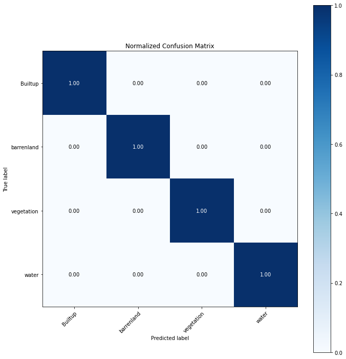
# predict on X_test to evaluate the model
preds = lgbm.predict(X_test)
cm = confusion_matrix(y_test, preds, labels=labels)
model_name = 'light_gbm.sav'
pickle.dump(lgbm, open(op.join(root_dir, model_name), 'wb'))
# match the pretrained model weight with the saved model above
model_name = 'light_gbm.sav'
# helper function for calculating ND*I indices (bands in the final dimension)
def band_index(arr, a, b):
return np.expand_dims((arr[..., a] - arr[..., b]) / (arr[..., a] + arr[..., b]), axis=1)
lgbm = pickle.load(open(op.join(root_dir, model_name), 'rb'))%%time
# open connections to our input and output images
# new_image = op.join(root_dir, 'Trans_nzoia_2019_10-04.tif')
raster_file = 'W__Home_hahmad_public_temp _project_landsat_train sample_sentinel_mosaic-Trans_Nzoia.tif'
new_image = raster_file
output_image = op.join(root_dir, "lgbm_classification.tif")
with rasterio.open(new_image, 'r') as src:
profile = src.profile
profile.update(
dtype=rasterio.uint8,
count=1,
)
with rasterio.open(output_image, 'w', **profile) as dst:
# perform prediction on each small image patch to minimize required memory
patch_size = 500
for i in range((src.shape[0] // patch_size) + 1):
for j in range((src.shape[1] // patch_size) + 1):
# define the pixels to read (and write)
window = rasterio.windows.Window(
j * patch_size,
i * patch_size,
# don't read past the image bounds
min(patch_size, src.shape[1] - j * patch_size),
min(patch_size, src.shape[0] - i * patch_size)
)
data = src.read(window=window)
# read the image into the proper format, adding indices if necessary
img_swp = np.moveaxis(data, 0, 2)
img_flat = img_swp.reshape(-1, img_swp.shape[-1])
img_ndvi = band_index(img_flat, 3, 2)
img_ndwi = band_index(img_flat, 1, 3)
img_w_ind = np.concatenate([img_flat, img_ndvi, img_ndwi], axis=1)
# remove no data values, store the indices for later use
# a later cell makes the assumption that all bands have identical no-data value arrangements
m = np.ma.masked_invalid(img_w_ind)
to_predict = img_w_ind[~m.mask].reshape(-1, img_w_ind.shape[-1])
# predict
if not len(to_predict):
continue
img_preds = lgbm.predict(to_predict)
# add the prediction back to the valid pixels (using only the first band of the mask to decide on validity)
# resize to the original image dimensions
output = np.zeros(img_flat.shape[0])
output[~m.mask[:,0]] = img_preds.flatten()
output = output.reshape(*img_swp.shape[:-1])
# create our final mask
mask = (~m.mask[:,0]).reshape(*img_swp.shape[:-1])
# write to the final file
dst.write(output.astype(rasterio.uint8), 1, window=window)
dst.write_mask(mask, window=window)
# write to the final file
dst.write(output.astype(rasterio.uint8), 1, window=window)
dst.write_mask(mask, window=window)CPU times: total: 52.4 s
Wall time: 25.3 s%%time
# Load the classification
if os.path.exists(op.join(root_dir, "lgbm_classification.tif")):
output_image = op.join(root_dir, "lgbm_classification.tif")
else:
output_image = 'lgbm_classification.tif'
def linear_rescale(image, in_range=(0, 1), out_range=(1, 255)):
imin, imax = in_range
omin, omax = out_range
image = np.clip(image, imin, imax) - imin
image = image / np.float(imax - imin)
return image * (omax - omin) + omin
with rasterio.open(output_image, 'r') as class_raster:
# show(class_raster)
lgbm_classes = class_raster.read()
# Load the original image
with rasterio.open(raster_file, 'r') as s2_raster:
# show(s2_raster)
s2 = s2_raster.read([1,2,3])
# Compare side by side
fig, (ax1, ax2) = plt.subplots(ncols=2, nrows=1, figsize=(10, 4), sharey=True)
show(lgbm_classes, transform=class_raster.transform, ax=ax1, title="lgbm Classes")
show(s2[[2,1,0], : , :], transform=s2_raster.transform, adjust='linear', ax=ax2, title="Sentinel 2 RGB")Clipping input data to the valid range for imshow with RGB data ([0..1] for floats or [0..255] for integers).CPU times: total: 1.22 s
Wall time: 2.09 s<AxesSubplot:title={'center':'Sentinel 2 RGB'}>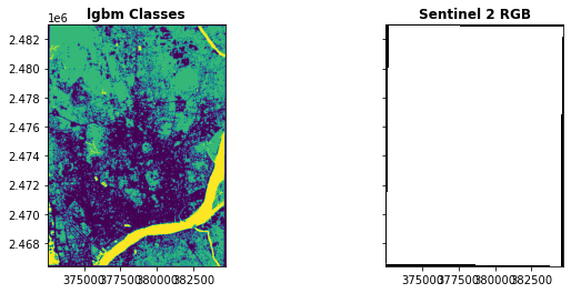
# Based on the histogram we'll set a threshold and rescale the data for visualization
# The values used for in_range are going to depend on the datatype and range of your data
# If you got the data from GEE try in_range(0, 2500)
for band in range(s2.shape[0]):
    s2[band] = linear_rescale(
            s2[band],
            #in_range=(0, 0.25),
            in_range=(0, 2500),
            out_range=[0, 255]
        )
s2 = s2.astype(np.uint8)
<timed exec>:12: DeprecationWarning: `np.float` is a deprecated alias for the builtin `float`. To silence this warning, use `float` by itself. Doing this will not modify any behavior and is safe. If you specifically wanted the numpy scalar type, use `np.float64` here.
Deprecated in NumPy 1.20; for more details and guidance: https://numpy.org/devdocs/release/1.20.0-notes.html#deprecations# Now retry the plot
fig, (ax1, ax2) = plt.subplots(ncols=2, nrows=1, figsize=(10, 4), sharey=True)
show(lgbm_classes, transform=class_raster.transform, ax=ax1, title="lgbm Classes")
show(s2[[2,1,0], : , :], transform=s2_raster.transform, adjust='linear', ax=ax2, title="Sentinel 2 RGB")<AxesSubplot:title={'center':'Sentinel 2 RGB'}>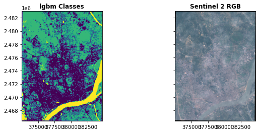
from matplotlib import colors
from matplotlib import cm

with rasterio.open(output_image, 'r') as rf_class_raster:
#  show(class_raster)
  rf_classes = rf_class_raster.read()

cls_colors = ['#ba0d11',


              '#ffa718',
              '#6fba4a',
              '#2b83ba']
clr_land = colors.ListedColormap([colors.hex2color(x) for x in cls_colors])


fig, (ax1) = plt.subplots(ncols=1, nrows=1, figsize=(12, 6), sharey=True)

im1 = ax1.imshow(lgbm_classes.squeeze(), cmap=cm.Accent_r)
show(lgbm_classes,
     transform=class_raster.transform,
     ax=ax1,
     title="lgbm Classes",
     cmap=clr_land
     )
# Now make a colorbar
norm = colors.BoundaryNorm(np.arange(0,5), clr_land.N)
cb = plt.colorbar(cm.ScalarMappable(norm=norm, cmap=clr_land), ax=ax1, fraction=0.03)
cb.set_ticks([x+.8 for x in range(0,4)]) # move the marks to the middle
cb.set_ticklabels(list(class_dict.keys())) # label the colors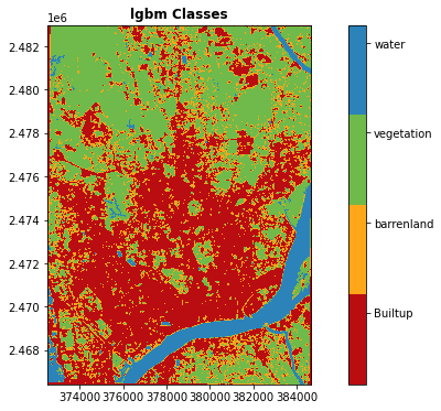
np.arange(0,4)array([0, 1, 2, 3])class_dict{'BarrendLand': 0, 'Builtup': 1, 'Forest': 2, 'Waterbodies': 3}